In RNA-Seq differential expression analysis, statistical models based on the negative binomial distribution, such as DESeq2 and edgeR, are widely used. On the other hand, t-tests are often described as “not suitable for RNA-Seq” or “inappropriate for count data.”
This explanation is useful as an introductory warning. In particular, it plays an important role in preventing misuse, such as applying a t-test directly to raw count values.
However, the explanation that “negative binomial models capture the structure of RNA-Seq data better than t-tests” has an important assumption. It applies when the target data are raw count values, or data in which low-expression genes and distributional distortions have not been sufficiently handled.
In raw count data, values are non-negative integers, and low-expression regions contain many 0s and 1s. The relationship between the mean and variance, as well as overdispersion, also cannot be ignored. Applying a t-test, which assumes a normal distribution, directly to such data is risky. In this sense, negative binomial models can be considered models that handle the properties of raw RNA-Seq count data more appropriately.
However, after appropriate normalization, preprocessing, filtering of low-expression genes, and visual inspection of data distributions and relationships among samples, this explanation can no longer be applied as-is. At that point, the data being analyzed are no longer raw count values themselves, but data that have been prepared in a form more suitable for statistical analysis.
For such data, simple comparisons such as “negative binomial models are essentially more correct” or “t-tests are inappropriate for RNA-Seq” become difficult to justify. Both should be treated as mathematical models for interpreting data, each with different assumptions and limitations.
What matters is not deciding in advance which statistical method to use, but checking the state of the data, understanding the effects of preprocessing and filtering, and interpreting the results based on what each method assumes and evaluates.
Why Did t-tests Come to Be Avoided in RNA-Seq Analysis?
The reason t-tests came to be avoided in RNA-Seq analysis is not only a matter of mathematical superiority, but also a practical one.
When RNA-Seq first became widely used, there were many cases where general statistical tests were applied to raw counts or inappropriately processed data without sufficiently accounting for low-expression genes, count data with many 0s and 1s, differences in library size, and overdispersion.
When a simple t-test is applied to such data, the results can be strongly distorted by unstable values in low-count regions, differences in library size among samples, and variance that depends on the mean expression level.
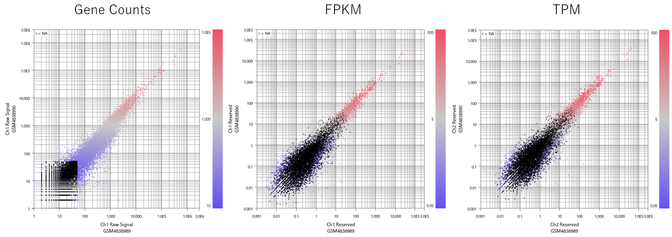
The spread of RPKM and FPKM also made this problem harder to recognize. Because RPKM and FPKM are values corrected for library size and gene length, they can appear to be “normalized expression values” that can be directly used for statistical analysis.
However, converting values to RPKM or FPKM does not make the original low-count values more reliable. Even when the raw count difference is only 1 versus 2, the transformed values may appear as a two-fold difference. Such differences may strongly reflect measurement uncertainty and sampling noise.
In other words, RPKM and FPKM do not solve the instability of low-count regions. Instead, they can make that instability appear like “normalized continuous values.” As a result, when general statistical tests such as t-tests are applied to RPKM or FPKM, unstable differences derived from low-expression genes may be treated as overly meaningful differences.
Later, TPM appeared and became more commonly used in place of FPKM and RPKM. TPM has the advantage of being easier to compare across samples than FPKM. However, TPM does not fundamentally solve the problem discussed here.
Even after conversion to TPM, problems such as instability derived from low counts, expression-dependent variance, and variability under small-sample conditions do not disappear. Therefore, it does not mean that TPM can simply be used as input for general statistical tests. Also, using TPM as input for a negative binomial model is outside the assumptions of the model and is inappropriate.
To avoid such misuse, RNA-Seq-specific statistical models such as DESeq2 and edgeR came to be widely recommended. These tools can handle low-expression genes, library size correction, expression-dependent variance, and variance estimation under small-sample conditions within a single analytical framework.
This trend was also supported by the practical efficiency of being able to use Gene Counts directly as input. Applying a simple t-test directly to Gene Counts without preprocessing can easily lead to major errors. By contrast, RNA-Seq-specific models accept Gene Counts as input and process them within a defined analytical workflow, making them easier to incorporate into pipelines that process large datasets using standardized procedures.
This property contributed greatly to the standardization of RNA-Seq analysis. At the same time, however, the sense of security that “standard models will handle the data if Gene Counts are provided” also became one reason why more analyses began to accept results without sufficiently checking the state of the data.
In this sense, the explanation that “t-tests should not be used directly for RNA-Seq” is reasonable as a safety-oriented warning for beginners. However, if it gradually turns into the simplified understanding that “t-tests are essentially inferior methods for RNA-Seq analysis,” the statement becomes inaccurate.
Understand Which Genes edgeR, DESeq2, and t-tests Tend to Identify—and Choose Methods Accordingly
As discussed above, caution is required when raw count values, RPKM/FPKM, or TPM
are used directly for statistical testing.
However, once low-expression genes have been removed,
data distributions and relationships among samples have been checked,
and normalization or log transformation has been applied,
the premise of the discussion changes.
At this stage, the data are no longer raw count values themselves,
but have already been prepared in a form more suitable for statistical analysis.
For such data, it is not possible to decide which method is essentially correct based only on names such as “t-test” or “negative binomial model.” No statistical model represents the true biological state exactly as it is. Each is an approximation for evaluating differences under specific assumptions.
At this point, the practical focus is not theoretical superiority, but understanding what kinds of genes a method tends to identify, and what kinds of genes it tends to miss. (Reference: How to Use edgeR, DESeq2, and t-test|Practical Rules by Data Type) Based on that understanding, it becomes important to consider how the genes of interest should appear, based on the biological background, clinical model, experimental system, and the experience and intuition of experimental biologists.
For example, the appropriate method and threshold strategy will differ depending on whether you want to focus on genes that change consistently but modestly in a disease model, genes that are strongly turned ON or OFF by treatment, or subtype-specific genes that respond strongly only in some samples.
Genes with high expression and consistent small differences among samples, genes with large Fold Changes but low and unstable expression levels, and genes that deviate strongly in only a subset of samples may be handled differently depending on the statistical method and preprocessing strategy.
Therefore, statistical methods are not devices that automatically produce the “correct answer.” They are tools for selecting candidate genes in light of the research purpose. In actual analysis, it is essential to examine what kind of gene list a method tends to produce, and whether that list fits the research objective and biological hypothesis.
On the other hand, the genes that biologists are truly looking for do not always appear as statistically significant differential expression. In particular, causal genes, or genes that are not causal themselves but are related to upstream pathways, may show mixed high and low expression patterns in both healthy and disease groups. (Reference: Why t-tests can work in practice even though they have theoretical limitations ) When searching for such genes, it can be useful to examine not only genes with strong significance, but also genes with higher P-values that are likely to be excluded from ordinary DEG lists, for example by checking them through clustering.
False positives can also be a problem with DESeq2 and edgeR
DESeq2 and edgeR are widely used standard methods for differential expression analysis based on RNA-Seq Gene Counts. However, using these methods does not always guarantee that false positives are properly controlled.
In fact, a study using large-scale RNA-Seq datasets from human population samples reported that DESeq2 and edgeR can detect more false positives than expected. In that study, the authors performed permutation analyses by shuffling condition labels and showed that DESeq2 and edgeR could still detect many differentially expressed genes, even in data where no true group difference should exist. (Reference: Exaggerated false positives by popular differential expression methods when analyzing human population samples)
The main causes discussed in that study include poor fit to the negative binomial model, the influence of outliers, and deviation from expected FDR control. Subsequent discussions have also pointed out that suppressing outliers by winsorization can reduce false positives, and that artificial false positives can be introduced in simulations when the impact of normalization is ignored.
However, these discussions do not mainly treat the shift in the lower bound of the low-count region on the left side of normalized histograms as a primary cause. In other words, they do not focus on differences in the effective detection limit among samples. In our own analyses of multiple datasets deposited in GEO, however, we have confirmed that this issue can affect the results of differential expression analysis. (Case studies: No.426 (an example of a level commonly observed in medium-sized datasets), No.403 (an example of a level that can strongly distort the analysis results))
Our point is not that t-tests should be rejected, nor that DESeq2 or edgeR should be rejected. Rather, whichever method is used, it is important to understand what view of the data the method assumes, what kinds of expression patterns are more likely to be selected by that method, and to choose the method appropriately according to the state of the data and the purpose of the study.
The Convenience of Modern Statistical Models Can Also Make Batch Effects Harder to Notice
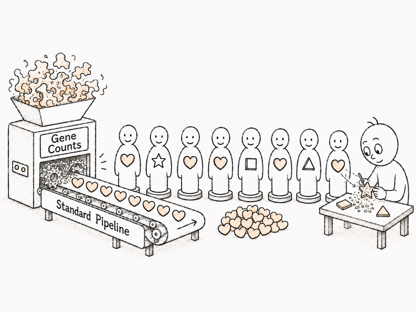
Modern statistical models such as DESeq2 and edgeR are highly useful. However, the convenience of obtaining differential expression results automatically from a standard pipeline simply by providing Gene Counts also creates another problem. That problem is that these methods may be used as standard procedures without sufficiently checking the state of the data.
As a result, analysis results that still include batch effects or biased sample composition may be treated as statistically well-organized DEG lists. In this sense, the risk may actually increase. The importance of checking PCA plots and expression distributions before concluding that a pattern is a batch effect is discussed in detail in another case study: What to check before calling it a batch effect .
Manually Inspecting Data Is Not an Outdated Approach
Manually checking data during analysis is not simply an old or inefficient approach. Rather, it is a necessary process for noticing batch effects, outliers, and biases in sample composition while proceeding with the analysis.
In an analysis workflow where data are checked step by step, you can examine distributions before and after normalization, the effects of low-expression genes, sample separation in PCA, clustering patterns, and expression patterns of individual genes.
For example, even when samples appear separated by experimental date rather than condition in PCA, this does not mean that a correction algorithm should simply be applied. There are many things to check, and that process cannot be replaced by automated processing.
Statistical models cannot be applied blindly to every dataset or purpose, and they may automatically exclude candidate genes that appear biologically important and deserve closer inspection .
Manually inspecting data is not about denying statistical models. A realistic and reliable analysis strategy is to combine automation based on statistical models with visual inspection by researchers themselves.
Examine the RNA-Seq Data Yourself
The idea discussed in this article—avoiding overreliance on statistical models and making decisions by looking at the data—is presented as a practical workflow in the RNA-Seq Data Analysis Tutorial | Learning the Analysis Workflow and How to Interpret Results Using GEO Data.
The tutorial covers importing Gene Counts, normalization, filtering, PCA, clustering, differential expression analysis, and enrichment analysis while checking the state of the data at each step. For a more practical example of using edgeR and DESeq2, see Differential Expression Analysis with edgeR and DESeq2 Using ChatGPT, which shows how to export Gene Counts from Subio Platform, generate an R script with ChatGPT, perform the analysis, and then import the results back into Subio Platform for visualization and validation.
Gaining hands-on experience in examining data helps researchers understand the characteristics of RNA-Seq data and the behavior of different analysis methods, and provides a foundation for thinking about subsequent automation strategies. This perspective is useful not only for experimental researchers, but also for bioinformaticians who design analysis pipelines and computational systems.