Many RNA-Seq and microarray datasets are publicly available in GEO. At first glance, combining multiple datasets may seem like a straightforward way to analyze a larger number of samples.
However, in practice, simply integrating multiple GEO Series often does not work well. Instead of separating by disease status or biological condition, samples often cluster according to the Series they came from.
This problem is not limited to the reanalysis of public GEO datasets. Even in your own RNA-Seq studies, data generated this year, next year, and several years later are not guaranteed to be directly comparable.
In this article, we use multiple GEO Series as an example to introduce the idea of integrating comparisons defined within each dataset, rather than integrating expression values themselves. We also discuss what this idea implies for the design of long-term prospective studies.
RNA-Seq Gene Counts Are Not Directly Comparable Absolute Values
RNA-Seq analysis produces Gene Counts, which represent how many reads are assigned to each gene. For those who are not familiar with expression data analysis, Gene Counts may look like absolute values that can be compared directly across datasets.
However, this is a major misunderstanding that many people encounter when they first work with RNA-Seq data.
Gene Counts do not simply represent how many RNA molecules were present in the sample.
Even when the same sample is measured, the count value for the same gene can change substantially
depending on measurement conditions and data processing.
This does not necessarily mean that the experiment was poorly performed.
Even when experienced technicians carefully follow the same protocol,
small differences in measurement batch, reagent lot, instrument, library preparation, or data processing
can change the scale and distribution of the count values.
This is a property that should be assumed from the beginning when working with RNA-Seq data.
Therefore, the possibility that samples from different GEO Series can be directly compared
as Gene Counts or normalized expression values is extremely low.
This is a basic premise in RNA-Seq data analysis.
On the other hand, if ratios are calculated against a control within the same Series,
comparisons across Series may become possible.
Expression values themselves may not be directly comparable, yet ratios can sometimes be compared.
This is an interesting property of RNA-Seq data.
In this article, we examine this idea using actual GEO datasets.
What Happens When Multiple GEO Series Are Integrated As They Are?
In this example, we used multiple GEO Series of skin samples from patients with Atopic Dermatitis (AD). As RNA-Seq datasets, we used GSE65832, GSE121212, and GSE140227. All of these datasets contain non-lesional and lesional skin samples from AD patients.
For Gene Counts, we used GEO Generated data for all Series. Using GEO Generated Gene Counts allows us to align the data processing pipeline to some extent. Even so, the expression value distributions differed substantially among the Series. These differences likely reflect differences in sequencer, sample condition, read depth, and other factors.
GSE65832, in particular, was generated using the older Illumina Genome Analyzer IIx platform and appears to have been derived from FFPE samples. In this Series, the typical bimodal distribution separating low-count and high-count regions, as seen in GSE121212 and GSE140227, is not clearly observed. At this point, it is already expected that integrating GSE65832 with the other Series as raw expression values would be very difficult.
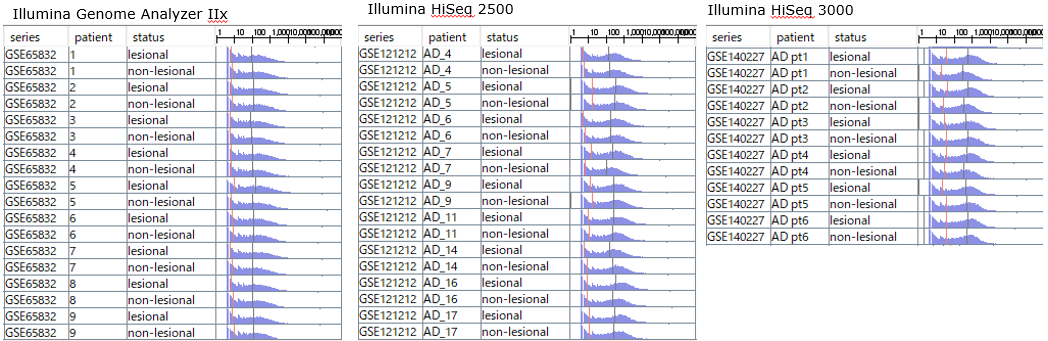
Distribution of gene count-derived expression values in GSE65832, GSE121212, and GSE140227.
GSE65832 was generated using Illumina Genome Analyzer IIx, GSE121212 using Illumina HiSeq 2500,
and GSE140227 using Illumina HiSeq 3000.
When these Series were integrated as they were and hierarchical clustering was performed, the differences among Series were reflected more strongly than the differences between lesional and non-lesional samples. In particular, GSE65832 was, as expected, far separated from the other two Series and appeared as an almost inverted expression profile. This shows how strongly technical differences between Series can be reflected when different RNA-Seq Series are simply combined.
The statement “samples from different Series cannot be directly compared” may be difficult to understand from words alone. However, this figure makes the meaning more intuitive. In this state, technical differences between Series are reflected much more strongly than the biological differences among samples.
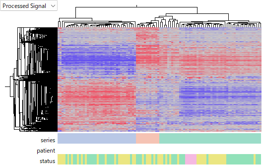
Hierarchical clustering of AD samples from GSE65832, GSE121212, and GSE140227 after integrating gene count-derived expression values as they are. In the Series color block, blue indicates GSE65832, pink indicates GSE140227, and green indicates GSE121212. In the status color block, green indicates non-lesional, yellow indicates lesional, and pink indicates chronic lesion.
Ratios Against Non-lesional Samples Within Each Series Reveal Cross-Series Comparisons
Next, each sample was converted into a log2 ratio using the average of the non-lesional samples within each Series as the reference. In other words, instead of correcting GSE65832, GSE121212, and GSE140227 using a single average across all Series, we used the non-lesional samples measured within each Series as the reference.
Compared with integrating expression values as they were, the separation by Series became weaker. Furthermore, we began to see patterns that were shared to some extent across Series: which genes were upregulated and which genes were downregulated in lesional or chronic lesion samples relative to non-lesional samples.
GSE65832 is especially worth noting. In the previous clustering, GSE65832 was far separated from the other two Series and appeared almost like an inverted expression profile. However, after transformation into log2 ratios using non-lesional samples within each Series as the reference, GSE65832 also began to appear as a similar expression-change pattern to the other two Series. This is a major step forward.
Of course, this method does not completely eliminate the differences among Series.
From here, batch-correction algorithms such as ComBat could be used to make the differences among Series appear smaller. However, this does not guarantee that the result is closer to the true biological state. Even if the clusters look cleaner, biological differences may be weakened together with batch effects, or artificial patterns may be introduced.
Therefore, even when correction algorithms are used, it is necessary to examine what changed before and after correction, rather than assuming that the result is correct simply because the samples appear to mix well.
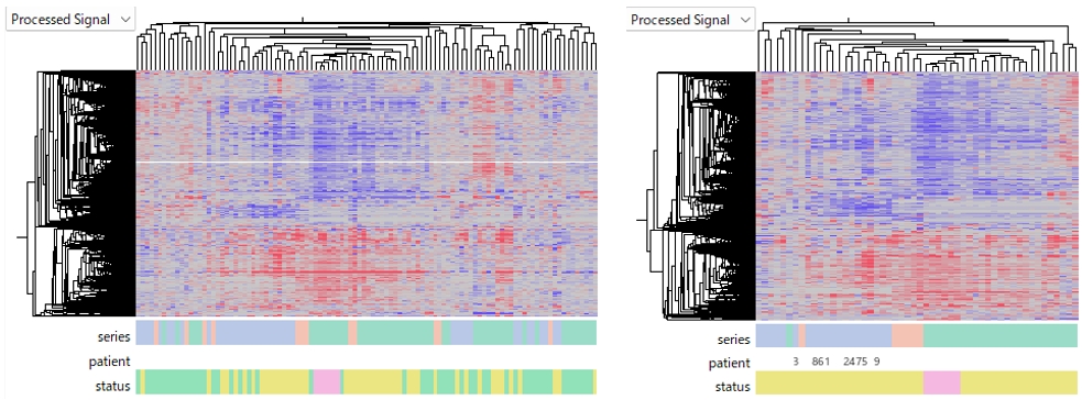
Hierarchical clustering after converting each sample into a log2 ratio using the average of non-lesional samples within each Series as the reference.
The left panel shows all samples including non-lesional samples, while the right panel shows only lesional and chronic lesion samples after excluding non-lesional samples.
In the Series color block, blue indicates GSE65832, pink indicates GSE140227, and green indicates GSE121212.
In the status color block, green indicates non-lesional, yellow indicates lesional, and pink indicates chronic lesion.
In the left panel, non-lesional samples and lesion samples (lesional / chronic lesion) each form clusters to some extent across Series.
Using Paired Non-lesional Samples From the Same Patient Can Reduce Individual Differences
The Series used here also contained pairs of non-lesional and lesional samples, or non-lesional and chronic lesion samples, obtained from the same patients. We therefore converted each lesional or chronic lesion sample into a log2 ratio using the paired non-lesional sample from the same patient as the reference.
This transformation reduces the baseline expression profile differences among patients. As a result, the analysis can focus not on inter-individual differences, but on how each sample changes from non-lesional to lesional or chronic lesion within the same patient.
In this clustering, only lesional and chronic lesion samples are shown. By using each patient’s paired non-lesional sample as the reference, not only differences among Series but also patient-specific background differences were further reduced, making lesion-associated expression changes more directly comparable.
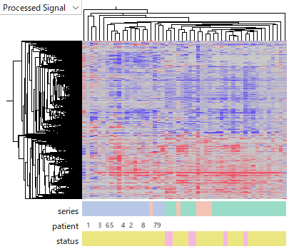
Hierarchical clustering after converting lesional or chronic lesion samples into log2 ratios using paired non-lesional samples from the same patients as references. Only lesional and chronic lesion samples are shown after excluding non-lesional samples. In the Series color block, blue indicates GSE65832, pink indicates GSE140227, and green indicates GSE121212. In the status color block, yellow indicates lesional and pink indicates chronic lesion.
When integrating multiple GEO Series, it is uncommon to have paired non-lesional and lesional samples from the same patients in this way. However, if such pairs are available, baseline expression differences among patients can be removed, allowing the analysis to focus on lesion-associated changes. This result shows how powerful a paired control can be as a correction strategy.
When paired samples are not available, the next key question is whether each Series contains a control group that can be used as a reference for comparison. However, multiple Series do not always contain control groups with the same biological meaning. The presence of such a control group itself is a valuable condition in integrative analysis.
Microarray Data Can Also Be Placed in the Same Analysis Space as Changes
Next, we added GSE36842, an Affymetrix HG-U133 Plus 2.0 microarray dataset. In GSE36842, acute lesional skin (ALS) was treated as “lesional,” and chronic lesional skin (CLS) was treated as “chronic lesion.”
Microarray and RNA-Seq data differ greatly in expression-value units, distributions, and dynamic ranges. Therefore, it is not appropriate to integrate microarray signal values and RNA-Seq Gene Counts or CPM as expression values in a single matrix.
However, when lesional or chronic lesion samples are converted into log2 ratios using paired non-lesional samples from the same patients as references, the comparison is no longer about expression values themselves. Instead, it represents how each patient’s sample changes toward the lesion state. In this form, it may be possible to explore shared expression changes across measurement technologies, including RNA-Seq and microarrays.
In fact, even after adding GSE36842 to the clustering, the direction of change appeared broadly consistent with the RNA-Seq data. Because GSE36842 uses processed data quantified by RMA, its range of variation appears much narrower than the log2 ratios derived from RNA-Seq. Even so, the overall direction of genes upregulated and downregulated in lesion samples was consistent with the RNA-Seq results.
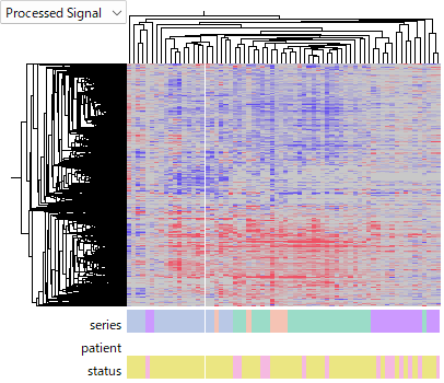
Hierarchical clustering after adding the Affymetrix HG-U133 Plus 2.0 microarray dataset GSE36842 to the RNA-Seq datasets. Lesional or chronic lesion samples were converted into log2 ratios using paired non-lesional samples from the same patients as references. In the Series color block, blue indicates GSE65832, pink indicates GSE140227, green indicates GSE121212, and purple indicates GSE36842. In the status color block, yellow indicates lesional and pink indicates chronic lesion.
This property was not newly discovered in the RNA-Seq era. Even in the microarray era, it was difficult to directly integrate expression values from different platforms, whereas fold changes or ratios obtained from the same comparison were often treated as indicators that could be compared across platforms.
Indeed, in the large-scale MicroArray Quality Control (MAQC) project, multiple reference RNA samples were measured at multiple sites and on multiple microarray platforms. The project evaluated within-platform reproducibility and cross-platform concordance of differentially expressed genes. This is a representative example showing the usefulness of looking at changes derived from the same comparison, rather than expression values themselves.
In this analysis, even after adding Affymetrix microarray data to the RNA-Seq data, when the data were expressed as log2 ratios of lesional or chronic lesion samples against paired non-lesional samples, the direction of expression changes appeared broadly shared despite differences in dynamic range.
Even as measurement technology has shifted from microarrays to RNA-Seq, the transcriptomic data property that changes derived from the same comparison are more reproducible than expression values themselves appears to have been carried forward.
Do Not Integrate Expression Values. Integrate Comparisons.
From the results shown above, we can see that when integrating multiple datasets, the goal is not to force expression values themselves onto the same scale.
It is necessary to define reliable comparisons within each dataset and integrate those comparisons with one another. In other words, what should be integrated is not expression values themselves, but changes defined within the experiment.
Examples include comparisons such as:
- disease / control
- treatment / untreated
- after / before
- time X / time 0
- differentiated / undifferentiated
- stimulated / unstimulated
When these comparisons are appropriately defined within each dataset, log2 ratios or differences may enable comparisons across Series or even across platforms.
However, this method does not work in every situation. Even after conversion to ratios, samples may still separate by Series. Even so, if each dataset contains samples that can be used as common controls, it is worth trying.
Preparing Ratio References as a Way to Handle Batch Effects
So far, we have looked at an example of integrating multiple GEO Series. However, the lesson here is not limited to the integration of public datasets. It can also be considered a more general strategy for handling batch effects.
Batch effects are systematic differences caused not by the biological differences we want to study, such as disease status or treatment condition, but by differences in measurement timing, sequencer, library preparation kit, reagent lot, sample preparation condition, analysis pipeline, and other factors. When these differences are large, samples appear to separate not by biological status, but by the Series or batch in which they were measured.
Batch-correction algorithms can be used to address such batch effects. However, completely correcting batch effects is not easy in practice. Therefore, rather than relying only on correction algorithms, it is safer to build countermeasures into the experimental design before data are generated.
One concrete approach is to include samples that serve as “ratio references” in each batch. Here, “control” does not necessarily mean a healthy sample against a disease sample, or an untreated sample against a treated sample. Rather, it means a reference sample for integrative analysis, used to compare data generated in different batches or at different time points later.
This reference sample needs to express the genes of interest at a sufficient level. If a gene is barely expressed in the reference sample, the ratio becomes unstable, and even small measurement errors can appear as large log2 ratios.
If a reference sample is included within the same batch, each sample can be expressed as a ratio or difference relative to that reference. Instead of directly comparing absolute expression values across batches, we can compare how each sample changes relative to the reference sample measured in the same batch.
In Prospective Studies, Build Future Comparability Into the Experimental Design
This idea is especially useful in prospective studies in which samples are collected over a long period. When patient enrollment or sample collection continues for several years, batch effects will inevitably become visible.
Samples measured this year and samples measured next year or several years later should be planned under the assumption that they cannot be directly compared as they are. Sequencers, library preparation kits, reagent lots, read length, read depth, analysis pipelines, measurement facilities, and operators will inevitably change over time.
First, the same reference sample should be included in each measurement batch. This allows newly measured samples in each batch to be expressed as ratios or differences relative to the reference sample.
In long-term studies, the consistency of the reference sample itself also becomes a problem, so additional precautions are needed. If the design depends on only one type of reference sample, changes in its storage condition, preparation lot, cellular state, or other properties may make the ratio reference itself unstable. Therefore, when possible, it is safer to prepare multiple reference samples with different properties.
The reference sample also needs to express the genes of interest at a sufficient level. If the research target has not yet been narrowed down, an artificial control sample designed to express as broad a range of genes as possible at sufficient levels may be useful.
What should be avoided in long-term studies is a situation where samples collected over several years can no longer be compared because of differences in measurement timing. Rather than trying to force expression values to match after the data have been generated, we should generate data in a form that preserves future comparability. This is a practical way to manage the risk of batch effects in prospective studies.
Supplement: Expression Values Are Inherently Ambiguous
As we have seen, the numerical values used in expression data analysis are strongly affected by batch effects. Or, more precisely, it may be better to think of them as values obtained through some measurement and processing conditions. In other words, Gene Counts and microarray signal values are not true expression levels themselves. They are observed values affected by measurement conditions and data processing.
Textbooks often explain that Gene Counts are affected by gene length, and that when comparing expression levels among different genes within the same sample, values such as TPM or FPKM should be used because they account for gene length and library size. Reading only this explanation, one might get the impression that TPM or FPKM are close to absolute expression values that can be compared both across genes and across samples.
However, the point to keep in mind is that TPM or FPKM do not reveal the true expression level itself. If Gene Counts are observed values affected by measurement conditions and data processing, then TPM and FPKM derived from them are also observed values affected by measurement conditions and data processing. In other words, even if a gene appears to have a certain expression level in one measurement, the same value is not guaranteed under different measurement conditions.
This also matters when interpreting databases that collect gene expression levels across many tissues or cell types. The fact that values are shown as TPM does not mean that they can be compared as absolute quantities. If the TPM value obtained from your own measurement does not match the TPM value listed in a database, that alone does not tell you which one is correct.