Standard RNA-Seq analysis workflows use PCA to examine overall gene expression profiles when assessing sample quality and potential batch effects. But do you stop at looking at the PCA plot in the QC report?
When some samples stand apart from the others, especially when the separation appears to align with the research question, it is tempting to interpret it as evidence of the expected biological difference. Before drawing conclusions, however, you need to investigate what underlies that separation and how much it affects the analysis results.
When the biological condition of interest overlaps completely with a technical factor, such as the experiment date, confounding may be easy to recognize. Real data, however, can be more complicated: multiple factors may overlap partially, or distinct sample groups may emerge within the same condition. When reanalyzing public data, detailed experimental information may also be unavailable. Even when these limitations make judgment difficult, it is important to keep investigating—comparing results with and without particular sample groups to work toward an analysis strategy and interpretation grounded in the data.
In this article, we use the public RNA-Seq dataset GSE173789, generated from CD19-positive B cells collected from healthy controls (HC) and patients with multiple sclerosis (MS). We investigate sample groups by moving between expression distributions, PCA, hierarchical clustering, and individual gene expression patterns. We then compare differential expression and enrichment analysis results across different sample subsets to examine how much the results—and the conclusions drawn from them—change depending on whether particular sample groups are included.
Below, we summarize the investigation presented in the video and discuss its implications. The analysis in this article uses the CPM data deposited in GEO by the original authors.
Examine the Distributions Rather Than Taking Normalized Values at Face Value
Subio Platform displays experimental parameters and histograms of value distributions in the same table. We examine the distribution of gene expression values within each sample using histograms, then compare expression profiles across samples using PCA, hierarchical clustering, and line graphs. Moving between these views helps connect different aspects of the data.
In the public CPM data, some samples had few low CPM values, leaving an empty region on the left side of their histograms and producing distributions markedly different from those of other samples. CPM (Counts Per Million) scales gene counts according to library size. When the total count used for this calculation is very small, even a few gene counts translate into relatively large CPM values. As a result, nonzero values cannot occupy the lowest part of the CPM range, leaving an empty region on the left side of the histogram. This is a plausible explanation for the distribution patterns observed here.
Indeed, many of the samples that stood apart in PCA broadly corresponded to samples with relatively low read counts or small FASTQ files, as recorded in the Sequence Read Archive (SRA). Examples included MS-13, MS-16–MS-19, and HC-19. However, the correspondence was not one-to-one. The number of reads assigned to genes can depend not only on the total number of reads, but also on the proportion passing QC filtering, the mapping rate, and the gene assignment rate.
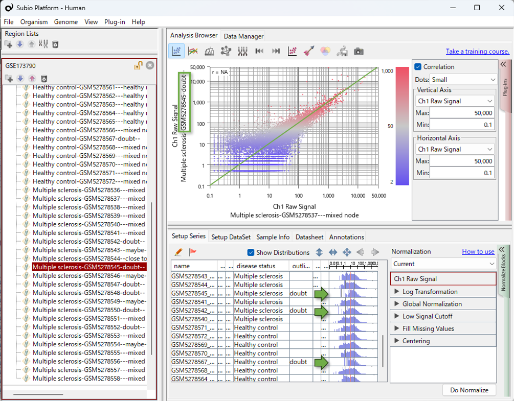
In this article, “distorted distributions” refers to expression-value distributions that differ markedly from those of other samples, particularly in having few values in the low-expression range.
Sample Composition Substantially Changes Differential Expression and Enrichment Results
How much does including or excluding these sample groups change the comparison between HC and MS?
In the video, we first identified seven samples that lay far from the others along PC1. We then identified six additional samples that clustered with them in the hierarchical clustering analysis and repeated the comparison after excluding all 13 samples. These included two HC samples and 11 MS samples, making this group heavily skewed toward MS. This imbalance introduced confounding into the HC–MS comparison, making it difficult to distinguish expression patterns specific to these samples from disease-associated expression differences.
Among the remaining 24 samples, six HC samples clustered together, separately from the other HC samples and the MS samples. Excluding these six samples as well again substantially changed which genes were identified as differentially expressed and which GO terms were enriched. Excluding the most conspicuous samples did not resolve the issue: a second pattern of sample separation became apparent, and it too influenced the results.
We used the same differential expression criteria and the same enrichment analysis settings across all three comparisons. The table below shows the sample sizes and the number of genes identified as more highly expressed in MS.
Changes in the Number of Upregulated Genes Across Sample Subsets
| Samples analyzed | HC samples |
MS samples |
Upregulated genes |
|---|---|---|---|
| All samples | 14 | 23 | 586 |
| Excluding 13 samples with distorted distributions | 12 | 12 | 1,297 |
| Excluding the above 13 samples and the cluster of six HC samples | 6 | 12 | 336 |
Upregulated genes: genes identified as more highly expressed in MS than in HC.
Only 54 genes were shared by all three upregulated gene lists. The GO terms—categories describing gene functions and related attributes—identified by enrichment analysis also changed with sample composition.
Excluding the 13 samples increased the number of upregulated genes from 586 to 1,297. Samples with distorted distributions may create apparent expression differences, but they may also obscure genuine differences. The increase in detected genes is therefore not inconsistent with an effect of distribution distortion. Excluding these samples may have allowed more genes with genuine expression differences to be detected. However, the increase alone does not establish that the resulting gene list is correct.
Excluding the six HC samples as well reduced the number of upregulated genes to 336 and changed both the gene list and the enrichment results. When these six samples are included, the HC–MS comparison also captures differences between these six samples and the rest. The genes identified as differentially expressed are therefore strongly influenced by the expression profiles of these six samples. After their exclusion, the remaining HC and MS samples have relatively similar expression profiles, with little differential expression. Here too, the distinct sample group was unevenly distributed across HC and MS, confounding the disease comparison and substantially influencing the results.
Both sample groups—the samples with distorted distributions, most of which were in the MS group, and the six HC samples with distinct expression profiles—substantially influenced the observed HC–MS differences. The resulting DEGs therefore cannot simply be interpreted as disease-associated expression changes. However, showing that a sample group strongly influences the results does not, by itself, justify excluding it. The available background information is insufficient for us to make a definitive decision about exclusion. Even so, comparing results across sample subsets and examining individual gene expression patterns can help us determine a reasonable analysis strategy.
In other datasets, samples that stand apart in PCA may have little effect on differential expression results. Their influence should therefore be assessed for each dataset. We can then investigate what might explain the characteristics of influential sample groups and decide how to handle them in light of the research question.
How Should We Interpret the Separate Cluster of Six HC Samples?
How should we interpret the cluster of six HC samples that became apparent after excluding the 13 samples with distorted distributions? These six samples clearly influence the results, but that alone does not tell us whether they should be excluded.
The IDs of these six samples, GSM5278560–GSM5278565, are consecutive. The combination of similar expression profiles and consecutive sample IDs gives us a reason to consider a possible batch effect. Before drawing that conclusion, however, we need to consider at least two possibilities.
Possibility 1: The Separation Reflects Biological Heterogeneity
The HC group may contain samples with different biological backgrounds, with those differences reflected in their expression profiles. Age, sex, inflammatory status, medical history, or the proportions of cell subsets might contribute. In this case, the separation within HC could contain information that is important to the analysis. These samples should therefore not be excluded without sufficient justification.
Possibility 2: The Separation Reflects Experimental or Technical Bias
Alternatively, the separation within HC may arise from library preparation, sequencing runs, sample processing dates, storage conditions, RNA quality, or other technical factors. In that case, the observed difference may reflect bias introduced during data generation or processing rather than a biological difference associated with disease.
Analysis Algorithms Alone Cannot Determine How to Proceed
Comparing different sample subsets reveals their influence on the results. It does not, however, automatically tell us which sample composition is appropriate for the research question. How we treat the cluster of six HC samples also depends on whether we interpret it as biological heterogeneity or technical bias.
In this situation, asking only “Which statistical method will solve this?” is not enough. A method may change how a structure appears without explaining its cause. Useful evidence includes the clinical backgrounds of the healthy controls, sample collection conditions, library preparation dates, sequencing runs, RNA quality, and laboratory records—information beyond the computational results.
When reanalyzing public data, this information may be incomplete, leaving some questions unresolved. Even then, comparisons across sample subsets can reveal which results change and which remain shared. We can then choose an analysis strategy based on the available evidence and state explicitly the assumptions underlying that strategy.
Similar Problems Recur in Other Public Datasets
In RNA-Seq analysis, following widely used tools and established protocols is often assumed to lead to more reliable results. Certainly, when researchers cannot fully evaluate the strengths and limitations of different tools themselves, their track records and reputations can provide useful guidance. In this original study, the GEO records indicate that the authors used the widely adopted edgeR package to convert gene counts into CPM values. They may also have used edgeR for differential expression analysis, although we have not been able to confirm this.
In any case, using standard tools does not guarantee the reliability of the results. Figures 4A and 4B of the original study also show sample patterns similar to those identified in our reanalysis. We could not find any discussion in the main text or supplementary materials examining how including or excluding these sample groups might affect the differential expression and enrichment analysis results.
In my experience reanalyzing public datasets, I have repeatedly encountered cases in which particular groups of samples substantially influence the results, yet their impact is not examined in the published studies. This recurring pattern led me to wonder whether broader, systemic factors might be involved, rather than simply a lack of attention on the part of individual researchers.
We therefore analyzed the same dataset using Galaxy, RaNA-Seq, RNAseqChef, and iDEP. By working through each tool, we examined the QC information and visualizations available at each stage, and how easily they could be used to investigate sample structure and its influence on the comparison results.
With Galaxy and RaNA-Seq, we reanalyzed the data starting from FASTQ files to generate gene counts. Their QC reports showed differences between samples in read counts and the number of reads assigned to genes. When we examined the resulting gene counts in Subio Platform, we also observed the distribution patterns seen in the public CPM data. These additional analyses followed the CPM-based investigation presented here.
Why might these sample structures go unnoticed in standard analysis workflows? And how easily can an analyst move from noticing a difference to testing its effect on the results? We explore these questions in the following articles:
- Using Galaxy
- Using RaNA-Seq (a closer look at the QC reports and gene counts)
- Using RNAseqChef
- Using iDEP
Further Investigation with Normalization and Batch Correction:
We further examined the sample structures observed in this case study using TMM, DESeq2 VST, quantile normalization, ComBat, and other approaches.
The Limits of Normalization and Batch Effect Correction in RNA-Seq
The Analyst’s Role
This article describes the observations and reasoning that emerged as I worked through this dataset. I do not claim that this is the only correct approach. What I want to convey is the importance of examining the data, considering multiple possibilities, making comparisons, and identifying where interpretations diverge.
When the evidence does not support a single interpretation, we need to organize the results under different scenarios and present them in a form that enables discussion with team leaders, experimental researchers, clinicians, pathologists, and others who understand the samples’ backgrounds.
Mastering advanced statistics is only part of omics data analysis. Visualizing the data, examining assumptions, and clearly explaining the data’s characteristics and the analysis results are also essential parts of the analyst’s work.
Learning to Analyze Data
Learning data analysis means building experience with diverse datasets: visualizing them, developing hypotheses, checking those hypotheses, and making judgments. This takes time, patience, and sustained practice.
How Subio Supports Your Development
Subio offers hands-on learning through online training , working with you on your own data. Although individual needs vary, around three to six one-to-one sessions over a year can help you steadily develop your approach to analysis and your ability to make informed judgments.
If you need results sooner, or would first like an expert assessment of your data, we recommend our data analysis service . This service goes beyond delivering a report. We help you understand the data’s characteristics and the analysis steps, then organize the evidence you need to make your own judgments and draw conclusions.
If you are interested, please contact us.
Learning commands and software tools is only part of the process.
What you ultimately need to learn is data analysis itself.
Related Topics
- RNA-Seq Data Analysis Tutorial | Learning the Workflow and How to Read Results Using GEO Data
- What Is RNA-Seq Differential Expression Analysis? | Beyond p-Values, edgeR, and DESeq2
- Omics Experiments Cannot Escape Nonlinear Bias
- Addressing Batch Effects in RNA-Seq | The Principle of Comparing Expression Changes Presented by MAQC 20 Years Ago