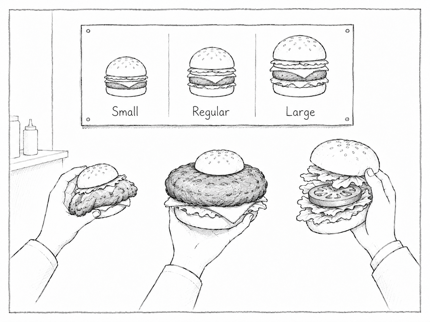
In RNA-Seq analysis, genes identified by differential expression analysis are often visualized in a heatmap. In such cases, instead of the original expression values, values converted to Z-scores for each gene or values scaled to a range from 0 to 1 may be used.
Because Z-score transformation and scaling are widely used as preprocessing steps for heatmaps, they may be assumed to be necessary for creating an RNA-Seq heatmap. However, they are not actually required.
This article explains what is preserved and what is lost through Z-score transformation and scaling. It then discusses why row scaling is often unnecessary for typical RNA-Seq datasets and may even reduce consistency across different analysis results. Cases in which row scaling may be necessary are also considered.
Terminology
For each row of a heatmap, the process of aligning the reference position, for example by subtracting the mean, is called centering. This removes differences in overall expression level among genes and makes it easier to focus on increases and decreases from the reference and on coordinated patterns among genes. Differences in the magnitude of variation among genes are preserved after centering. When log-transformed RNA-Seq values are centered, the focus shifts from absolute differences in expression level to relative changes from the reference value of each gene, that is, fold change.
By contrast, the process of using the standard deviation, the range of values, or another measure to equalize the magnitude of variation in each row is called scaling. In this article, scaling performed separately for each row of a heatmap is referred to as row scaling.
Common methods of row scaling include conversion to Z-scores and min–max scaling based on the minimum and maximum values.
In a Z-score transformation, the mean of each gene is subtracted to center the values, and the result is then divided by the standard deviation of that gene. As a result, each gene has a mean of 0 and a standard deviation of 1. Therefore, genes that originally showed only small variation and genes that showed large variation are displayed as having a similar degree of variation in the heatmap.
In min–max scaling, the minimum value of each gene is subtracted, and the result is then divided by the difference between the maximum and minimum values. As a result, the minimum value of each gene becomes 0 and the maximum becomes 1. For example, a change from 100 to 200 and a change from 100 to 10,000 are both transformed to the range from 0 to 1. In this article, this transformation is referred to as 0–1 scaling.
Note: Using VST or rlog Values in Heatmaps
VST and rlog, which are commonly used in RNA-Seq analysis, are different from the row scaling discussed here. These transformations reduce the dependence of variance on mean counts and help prevent the large variability observed in the low-count range from having an excessive influence on the analysis. When clustering or heatmaps are generated after applying VST or rlog, variation among genes in the low-count range tends to become less prominent. Therefore, when genes with low counts have been sufficiently filtered out, the difference between VST or rlog and a simple log transformation becomes smaller.
Whether VST or rlog is appropriate for a heatmap also depends on the method and values used for DEG analysis. In DESeq2, differential expression is tested using Counts, while VST and rlog are mainly used for clustering and visualization. They therefore provide a practical approximation for examining sample-level expression patterns among genes identified as DEGs. By contrast, when visualizing edgeR results, it is more natural to use an approximate display value that corresponds to edgeR normalization, such as logCPM calculated after TMM normalization. When a t-test or nonparametric test has been performed using log-transformed normalized values, TPM, or FPKM, using the same values in the heatmap provides greater consistency with the statistical test.
However, using such approximate values for visualization can make the relationship with the original Gene Counts and the dynamic range of each sample more difficult to see. Therefore, VST and rlog are not always the most appropriate values for visualization. The values used for display should be selected not only according to their relationship with the method and values used for DEG analysis, but also according to which features of the original data need to be examined.
In summary, VST and rlog are well suited for presenting sample-level expression patterns among genes identified as DEGs in an easily interpretable form. However, because they make the relationship with the original Gene Counts less visible, they may be less suitable for examining how the analysis results were produced.
Why Are Values Transformed Separately for Each Gene?
Expression levels differ greatly among genes. For example, suppose one gene varies within a gene count range of 1–10, while another varies within a range of 100–1,000. When a common color scale is used for all genes, differences in color mainly reflect differences in expression level, making the expression changes of individual genes difficult to see.
Centering is necessary to avoid this problem. However, is it also necessary to perform row scaling and equalize the magnitude of variation among genes?
Amplitude Is Important for Biological Interpretation
The magnitude of variation in RNA-Seq data is not merely a numerical difference.
The magnitude of a change in gene expression is important when considering the strength of a response and the potential scale of its biological effect. For example, even when two genes have the same p-value, a gene that changes by only 1.2-fold and a gene that changes by 10-fold may represent very different biological phenomena.
Amplitude Is Also Needed to Evaluate the Validity of Other Analysis Results
Information about amplitude is also needed to assess the validity of differential expression analysis and other analysis results. For example, when genes identified as DEGs are displayed in a heatmap, at least the following points should be examined.
- Whether the group difference seen in the mean values is also visible in the individual samples
- Whether the direction of change is reproduced across replicate samples
- Whether the difference is being driven by only a small number of samples
- Whether subgroups with different magnitudes of expression variation exist within the same experimental group
However, row scaling removes differences in the magnitude of change. As a result, differences such as those listed above may become difficult to see.
In addition, when multiple experimental groups are present, averaging the replicate samples within each group before drawing the heatmap removes information about within-group variation. Therefore, a heatmap that combines averaging with row scaling reduces, in two separate ways, the information needed to evaluate the validity of the DEG analysis.
Cases in Which Equalizing Amplitude Is Necessary Are Limited
Under what circumstances, then, is it reasonable to equalize the magnitude of variation?
In general statistical analysis, when variables with different units and different numerical ranges, such as height and body weight, are entered into the same multivariate analysis, their scales may need to be aligned so that variables with larger numerical ranges do not dominate the result. This is the most common reason why scaling is considered necessary.
Within a single RNA-Seq dataset, however, the expression values of different genes are generally obtained using the same measurement method, the same units, and the same analytical procedure. Differences in the magnitude of variation among genes contain information about expression level, response strength, measurement stability, and other characteristics. Therefore, there is usually little benefit in discarding such important information by applying row scaling.
Examples in which scaling may be necessary in RNA-Seq analysis include the following.
- Integrating multiple independent RNA-Seq datasets
- Integrating transcriptome datasets generated by different measurement methods, such as RNA-Seq, microarrays, and qPCR
- Integrating different types of omics datasets, such as transcriptomics, proteomics, and DNA methylation data
- Entering expression data and clinical laboratory measurements into the same analysis
Even in such cases, simply converting the values to Z-scores does not resolve differences between measurement methods or batch effects. Each dataset should first undergo appropriate normalization and quality assessment. Only after that should the scales be aligned, when necessary, according to the objective of the analysis and the downstream algorithm.
Similarly, when scaling is used as preprocessing for machine learning, the appropriate method depends on whether the downstream algorithm is affected by the scale of the input features.
Therefore, equalizing amplitude is not a general-purpose preprocessing step. It is a conditional option that depends on the purpose of the analysis and the downstream method.
Reanalyzing Fig. 5F of GSE95304
We will now examine Fig. 5F from a study using the public RNA-Seq dataset GSE95304. This dataset is also used as an example in another article. Here, however, the purpose is not to criticize the analytical approach or the logic of the paper, but to use it as a concrete example for considering a problem that is also common in RNA-Seq analysis more generally.
In this study, the transcription factors Fra-1, MYC, E2F1, TP53, and others were knocked down using shRNA, and the effects on gene expression were examined. In the paper, 295 genes were identified through an expression analysis using FPKM and displayed as a heatmap in Fig. 5F.
When the filters and statistical test described in the Methods were applied to the publicly available FPKM data, the number of genes was reduced from 23,615 to 12,239, and the same 295 genes satisfying FDR < 0.1 were reproduced. Among them, 157 genes showed lower expression and 138 showed higher expression in the knockdown group. Therefore, the process used to select the genes shown in Fig. 5F could be broadly reproduced from the public data.
The 295 Genes Were Not Genes That Were Significant for Each shRNA Separately
To understand what these 295 genes represent, it is necessary to confirm how they were selected. The 295 genes were not obtained by performing differential expression analysis separately for each shRNA and then taking the union of the results. Eight shSCR samples were treated as the control group, while two samples each for Fra-1, MYC, E2F1, and TP53 knockdown, for a total of eight samples, were combined as the knockdown group. An 8-versus-8 comparison was then performed. Therefore, what this test shows is that there was an average difference in expression between the group combining four types of knockdown and the shSCR group.
Fig. 5F Appears to Address a Different Question from the Statistical Test
In Fig. 5F, the 295 genes are displayed separately for each shRNA condition. In addition, the replicate samples for each condition were averaged, and 0–1 scaling was applied separately to each gene. However, the order in which averaging and scaling were performed is not clearly described. Regardless of the order of these operations, Fig. 5F may give the impression that genes individually affected by each shRNA were collected and that many of them showed coordinated changes across multiple shRNA conditions. The question answered by the differential expression analysis and the information that Fig. 5F appears to present to the reader do not completely match.
To confirm the group difference captured by this differential expression analysis using a heatmap, the visualization should use either the same values as the differential expression analysis or values subjected only to the minimum necessary transformations for visualization, namely log transformation and centering. The same samples used in the differential expression analysis should also be displayed individually.
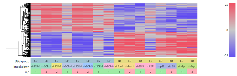
In this figure, the FPKM values used in the differential expression analysis were log-transformed and centered separately for each gene. The same 16 samples used in the differential expression analysis are arranged as eight control samples and eight knockdown samples, matching the two-group comparison used in the test. The samples are displayed individually without averaging. The upper annotation row, “DEG group,” shows the two groups used in the differential expression analysis. The shRNA condition and replicate number for each sample are shown below it. To preserve differences in the magnitude of variation among genes, row scaling was not applied.
For shFra-1, shp53, and shMyc, the two replicate samples show relatively similar expression patterns. By contrast, for shE2F1, the batch 2 sample shows a different expression pattern. It is possible that shE2F1 produces changes similar to those seen for the other three shRNAs, but this cannot be determined from the two available samples, and the conclusion should therefore remain open.
The control shSCR samples also do not all show a uniform expression pattern. In particular, differences are visible between batch 1 and batch 2.
When the individual samples are displayed in this way, it becomes apparent that the group difference among the 295 selected genes strongly reflects the difference between the four shSCR batch 2 samples and the seven knockdown samples excluding the shE2F1 batch 2 sample.
Importantly, even if this figure had been used instead of Fig. 5F, it would still support the central idea of the paper that some genes show common changes in response to multiple shRNA treatments. Rather, it would show the variation among individual samples and distinguish the knockdown conditions in which a common pattern can be confirmed from those in which the conclusion should remain open.
Consistency of Values Is Important When Relating Analysis Results
The issue discussed here is not limited to one particular visualization method. More generally, it concerns the basis on which multiple analysis results are related to one another and interpreted together.
RNA-Seq analysis often presents PCA, clustering, heatmaps, differential expression analysis, enrichment analysis, and other results as a single analytical flow. However, when these results are generated from different values, different sets of samples, or different gene-selection criteria, they do not necessarily represent the same information, even when they originate from the same dataset.
When multiple analysis results are interpreted together, it is clearer, wherever possible, to use the same values, the same samples, and the same set of genes. The more information the analyses have in common, the more directly it is possible to determine whether a feature observed in one result is also present in another.
On the other hand, different values or data-processing methods may be required because of the objectives of the analysis or the characteristics of the methods used. In such cases, it is necessary to clearly recognize what each processing step preserves, what it changes, and what it removes. When presenting the results, the values used and the processing applied to them should also be clearly stated.
Such confirmation is not always easy in analytical pipelines constructed by combining individual R tools or in software packages that automatically run multiple analysis tools. It may be difficult to determine which values were used to generate each result, and users may not notice that transformations they did not intend or were not aware of were applied during the workflow.
Therefore, the more automatically a series of analysis results is generated, the more important it becomes to examine not only whether each individual analysis was executed correctly, but also which values were used to generate each result and to what extent those results can legitimately be interpreted together. This issue is discussed in more detail in The Values Shown in a Heatmap and the Values Used for DEG Analysis May Not Be the Same .