RNA-Seq analysis commonly follows a series of steps that include FASTQ quality control, alignment, generation of Gene Counts, normalization, and detection of differentially expressed genes (DEGs). Galaxy allows users to run many commonly used RNA-Seq tools sequentially through a GUI. One of its major advantages is that users can follow a standard analysis workflow without having to build a command-line environment themselves.
But if we follow such a standard workflow and run each tool correctly, can we also determine whether the final analysis results are reliable? In this article, we examine this question using the GSE173789 dataset. In a previous case study, we confirmed that this dataset contains expression changes strongly suspected to have arisen from factors unrelated to the original biological objective of the study. Before continuing, we recommend first reading that case study or watching the short analysis video below to understand the characteristics of this dataset.
Short Instruction 1: Detecting Potential Outliers with PCA and Confirming Them with Multiple Visualizations
We then analyzed this clearly distorted dataset by following a standard Galaxy workflow and examined what could be detected at each step and how far we could go in assessing the validity of the final results. For the workflow, we referred to the Galaxy Training Network (GTN) tutorials RNA-Seq reads to counts and RNA-seq counts to genes.
In Galaxy, Attention Is Easily Drawn Toward Getting the Analysis to Run to Completion
One thing that became clear while using Galaxy was that RNA-Seq analysis is not completed within a single integrated tool. Instead, it involves connecting multiple tools step by step. FASTQ files are passed to FastQC, the results are summarized with MultiQC, paired-end data are passed to HISAT2, the resulting BAM files are passed to featureCounts, and the Gene Counts then have to be organized into a format that can be analyzed with limma.
In practice, many small problems arise along the way. In this analysis, we encountered problems even before the analysis itself began, during FASTQ retrieval. When we attempted to obtain FASTQ files from SRA accessions within Galaxy, fasterq-dump produced an error whose cause was not easy to identify from the user side. It was difficult to determine whether the problem originated from the data, NCBI, Galaxy, the network connection, or a temporary service issue. We were able to work around this by switching to fastq-dump.
There were also smaller tasks such as reorganizing collections so that FastQC results could be passed to MultiQC and adjusting data structures between tools. During HISAT2 alignment, two samples terminated with signal 9, and we could not find a way to resolve the problem. We therefore excluded those two samples from the analysis. That was acceptable for the purpose of this experiment, but if the goal had been publication, we would have needed to somehow resolve the issue.
These problems have to be addressed one by one before the analysis can move forward. As a result, attention naturally shifts toward questions such as, “Why did this job fail?”, “What format does the next tool require?”, and “How can I get the pipeline to finish?” Once those errors are resolved and the workflow finally reaches DEG analysis, it is easy to feel that the analysis itself has been successfully completed.
Today, AI assistance makes dealing with this kind of technical problem far easier than it used to be. Even so, our attention still tends to be drawn toward getting the analysis to run successfully from beginning to end, while the difficulty of deciding whether the resulting analysis can actually be trusted remains.
FastQC and MultiQC Provide a Great Deal of Information, but They Do Not Tell You Which Samples to Exclude
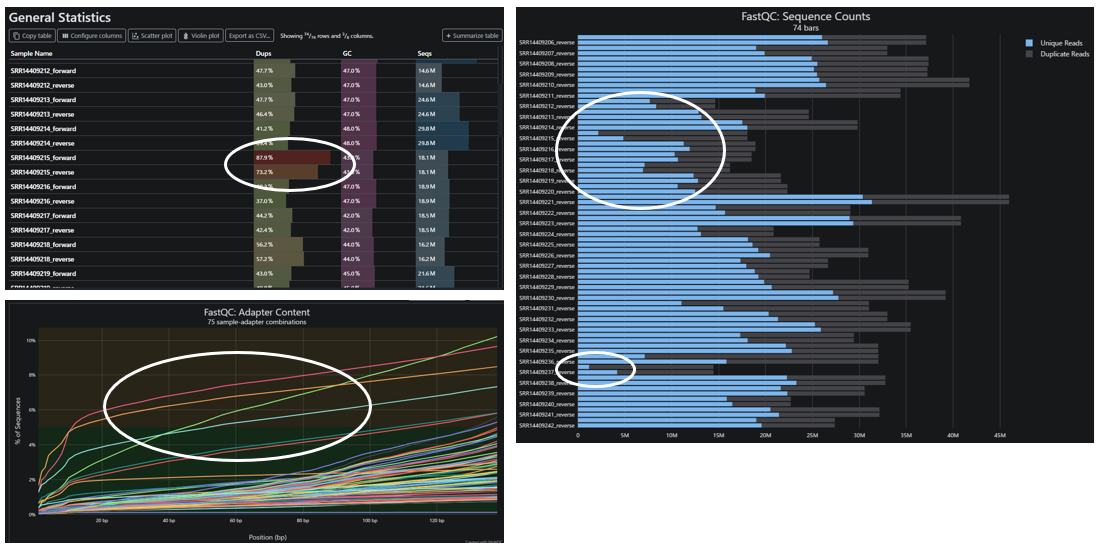
We first ran FastQC on all FASTQ files and summarized the results with MultiQC. This provides many QC metrics in one place, including Sequence Counts, Sequence Quality, Duplication, and Adapter Content. In this dataset, there were substantial differences in read counts between samples, and some samples also showed clearly different patterns in Duplication and Adapter Content.
We already knew that this dataset contained such variation and that it was strongly associated with the expression profiles, so we examined these results carefully. However, without that prior knowledge, it would not be possible to decide whether a sample should be excluded based on these reports alone. High Duplication does not necessarily indicate a problem in RNA-Seq data, and some degree of variation in read counts is expected. There is no universal threshold that tells us when such differences are large enough to materially affect the final results.
An experienced analyst might notice that something could be unusual in the QC results. A careful analyst might write down the IDs of suspicious samples and continue tracking them in later steps. But it is easy to imagine that someone performing this type of analysis for the first time might simply continue to the next step without giving them much attention.
Sample IDs Alone Make the Reports Much Harder to Interpret
Another thing we noticed was how strongly sample naming affects the interpretability of the results and reports. When FASTQ files were obtained from SRA accessions within Galaxy, the SRR accessions were used directly as the dataset names. As a result, when looking at MultiQC, featureCounts, or later MDS plots, names such as SRR14409217 and SRR14409222 did not immediately tell us whether a sample belonged to the MultipleSclerosis or HealthyControl group.
Of course, this information can be checked in a separate metadata table. But having to return to that table every time we compare reports from different stages makes the comparison considerably more cumbersome. In an analysis like this one, where we want to relate read counts, Count distributions, assignment rates, MDS positions, and DiseaseState, sample names that contain no information about the experimental conditions make interpretation considerably more difficult.
Whenever possible, it is better to retain the original ID while also including major experimental information in the sample label. For example,
SRR14409217_MS_sample01
would make reports much easier to understand.
However, when many SRA Runs are downloaded in bulk using tools such as Galaxy's built-in fastq-dump, manually renaming every generated dataset can be quite cumbersome. Even so, it is important to organize the relationship between sample IDs and experimental conditions before beginning the analysis and, where possible, assign informative sample labels early in the workflow.
featureCounts Also Provides Clues, but They Are Still Not Enough for Exclusion Decisions
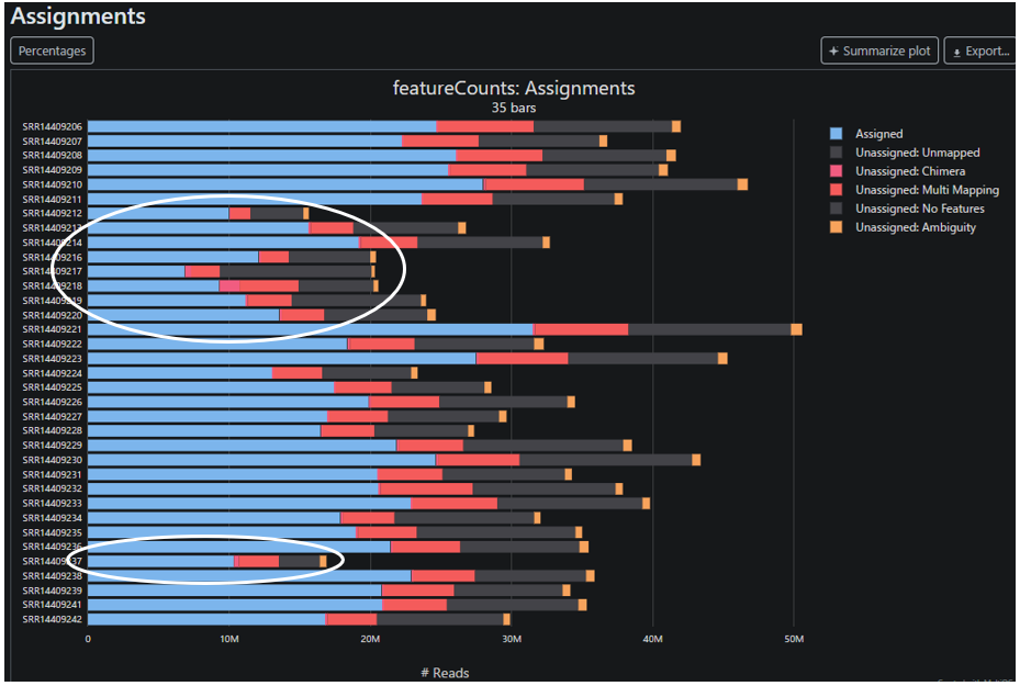
After running featureCounts, we examined the assignment rates with MultiQC. Most samples were in the range of approximately 55–64%, while several showed considerably lower values. However, once again, assignment rate alone was not sufficient to determine whether a sample should be excluded from the analysis. A low assignment rate did not necessarily correspond to the same pattern in the downstream expression distributions.
So here again, the report contains information worth noticing, but it is difficult to justify excluding a specific sample at this stage. Continuing to generate the Gene Counts and proceeding to the statistical analysis would be a natural choice.
The Data Still Made It to limma-voom
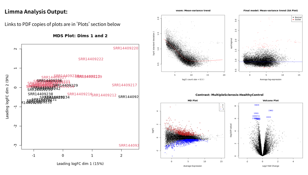
We combined the Gene Counts obtained from featureCounts and performed differential expression analysis with limma-voom. The comparison was MultipleSclerosis versus HealthyControl. Low-count genes were filtered based on CPM, followed by TMM normalization and voom mean-variance modeling.
The limma report includes an MDS plot, mean-variance trend, model fit, MD plot, Volcano plot, and other diagnostic outputs. These reports give no obvious indication that the analysis has failed. The mean-variance trend looks reasonable, and the Volcano plot shows many candidate differentially expressed genes. Using adjusted p-values to define DEGs, one could proceed directly to GO or pathway analysis.
The MDS plot also appears to show some separation between MultipleSclerosis and HealthyControl. If the plot is colored only by DiseaseState, it is natural to interpret this as indicating that the gene expression profiles of MultipleSclerosis and HealthyControl differ. By this point, the standard analysis has run to completion, the diagnostic plots do not show an obvious problem, and DEGs have been obtained. At this point, it is natural to feel confident in the result.
But When the Results Are Viewed Together with the Original Gene Counts, a Different Pattern Emerges
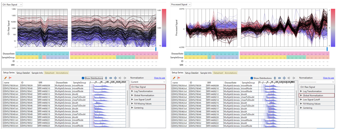
We therefore used Subio Platform to visualize the Gene Counts obtained from featureCounts together with the downstream analysis results. When we compare the original Gene Count distributions across samples, some samples clearly show substantially lower expression levels overall. When colored by SampleGroup, many of the samples classified as doubt or closeToDoubt fall among the samples with lower overall Count distributions. These are the same groups highlighted in the case study mentioned above.
After normalization, the differences in sample-level distributions become much smaller. Of course, normalization is necessary in RNA-Seq because library size and RNA composition differ between samples, and Gene Counts cannot simply be compared directly. The important question here is whether the differences seen after correction reflect biological differences, or whether they are related to technical differences that were already present in the original data.
Only when we examine together the variation in read counts seen in the FASTQ QC report, the differences in assignment rate from featureCounts, the distributions of the original Gene Counts, the changes introduced by normalization, and the MDS and DEG results do the relationships among these observations become apparent. At the very least, this allows us to examine problems that would not have been apparent from the final DEG results alone.
This Does Not Mean That limma Is Wrong
We are not trying to criticize Galaxy or limma-voom. limma is a tool that performs statistical analysis based on the expression data and experimental design that it is given. It evaluates group differences while accounting for factors such as library size and the mean-variance relationship, under the assumption that the input data are appropriate for the intended comparison.
However, data that reach limma do not necessarily satisfy those assumptions simply because they have passed through standard steps such as FastQC, HISAT2, and featureCounts. Completing those steps does not guarantee that the data are suitable for the final group comparison.
In other words, limma statistically analyzes the data it is given, but it does not determine whether those data should have been compared in the first place. That decision remains with the analyst.
Individual Tool Reports Do Not Show the Whole Analysis
FastQC evaluates FASTQ quality, featureCounts evaluates how reads are assigned to genes, and limma performs statistical analysis based on the expression matrix and design matrix it receives. Each tool provides information relevant to its own purpose.
However, none of these reports automatically shows, for example, whether a sample with a low read count in FastQC also has low Counts in featureCounts, where that sample lies in the limma MDS plot, and which DiseaseState it belongs to. In this analysis, information that did not look strong enough to change the analysis when viewed individually began to form a consistent pattern when it was examined together for the same samples.
What matters, therefore, is not simply generating more QC information, but being able to examine read counts, assignment rates, Gene Count distributions, changes after normalization, MDS, DEG results, and experimental conditions together for the same samples. This is also why reports became much harder to interpret when the samples were labeled only by SRR accession.
Even So, the Analyst Still Has to Make the Decision
Even when all of this information is viewed together, there is not always a single unambiguous answer as to whether a sample should be included or excluded. RNA-Seq data naturally contain substantial variation, and there is no universal boundary defining when a low read count, high Duplication, low assignment rate, or separation in MDS should be considered abnormal.
The problem becomes even more difficult when technical differences overlap with DiseaseState. In such cases, it may be difficult to determine whether an observed difference is biological, technical, or a combination of both. Even so, the analyst must ultimately decide whether the data should be included in the analysis and how much confidence should be placed in the results.
That is why the information needed for this decision should not remain fragmented across separate reports. Read counts, assignment rates, Gene Count distributions, changes introduced by normalization, MDS and DEG results, sample IDs, experimental conditions, and other relevant information need to be reviewed together. A way to review all of this information together is essential.
Running a Pipeline and Performing an Analysis Are Not the Same Thing
In a previous article, Can Different Values Be Used for Heatmaps and DEG Analysis in RNA-Seq?, we discussed a different problem: different tools may use fundamentally different values, yet the resulting figures can be presented together as though they were simply different visualizations of the same underlying information. In reality, those tools may be representing different aspects of the data.
The issue we encountered here with Galaxy is different. FastQC, featureCounts, limma, and the other steps each contain important information, but any single observation may not appear strong enough to justify excluding a sample or changing the analysis strategy. As a result, those clues may be treated as isolated variations and the workflow continues. Only when read counts, assignment rates, Count distributions, changes before and after normalization, MDS, DEG results, and experimental conditions such as DiseaseState are examined together for the same samples do those weak clues begin to form a coherent pattern.
These are different problems, but they share a common origin. RNA-Seq analysis is typically built by connecting tools that are individually well-established and designed for their respective purposes. Simply examining the output of each tool in sequence does not necessarily reveal what is happening across the analysis as a whole. The problem is not with the individual tools themselves, but with the fact that the need to integrate information across multiple stages and interpret the analysis as a whole is not sufficiently emphasized in current pipeline-based analysis.
This issue is not unique to Galaxy. The same applies when multiple tools and packages are combined in Bioconductor, Python, or other analysis environments. Traditionally, correctly running a predefined RNA-Seq pipeline and dealing with tool settings and errors has itself been considered an important skill for an analyst. But that alone is not analysis.
Running a pipeline and interpreting the information produced by that pipeline are different tasks. The former is becoming rapidly easier with AI and GUI-based tools. The latter remains the responsibility of the analyst. Integrating information obtained across multiple stages and interpreting it in the context of the analysis as a whole—that is the role of the analyst.
Related resources: If you would like to learn the complete RNA-Seq analysis workflow using real data, see our RNA-Seq Data Analysis Tutorial. To visualize results from different stages of the analysis and review them alongside the underlying data for validation, see Subio Platform.