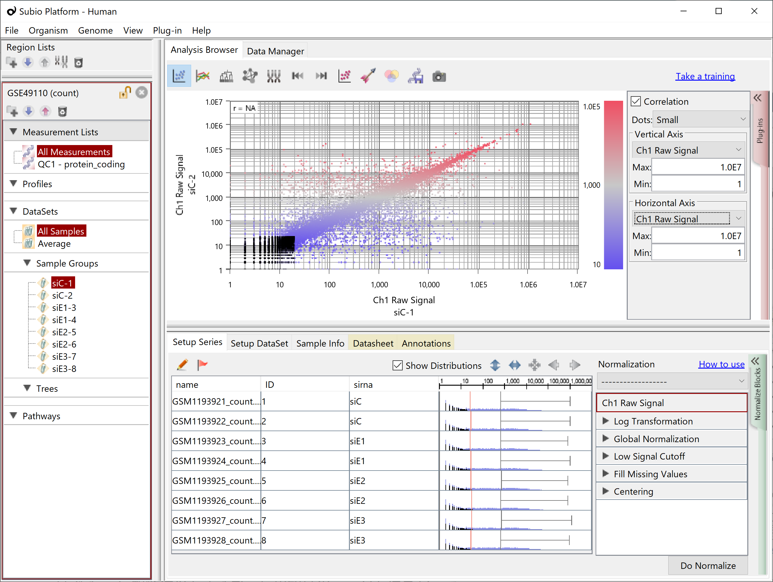
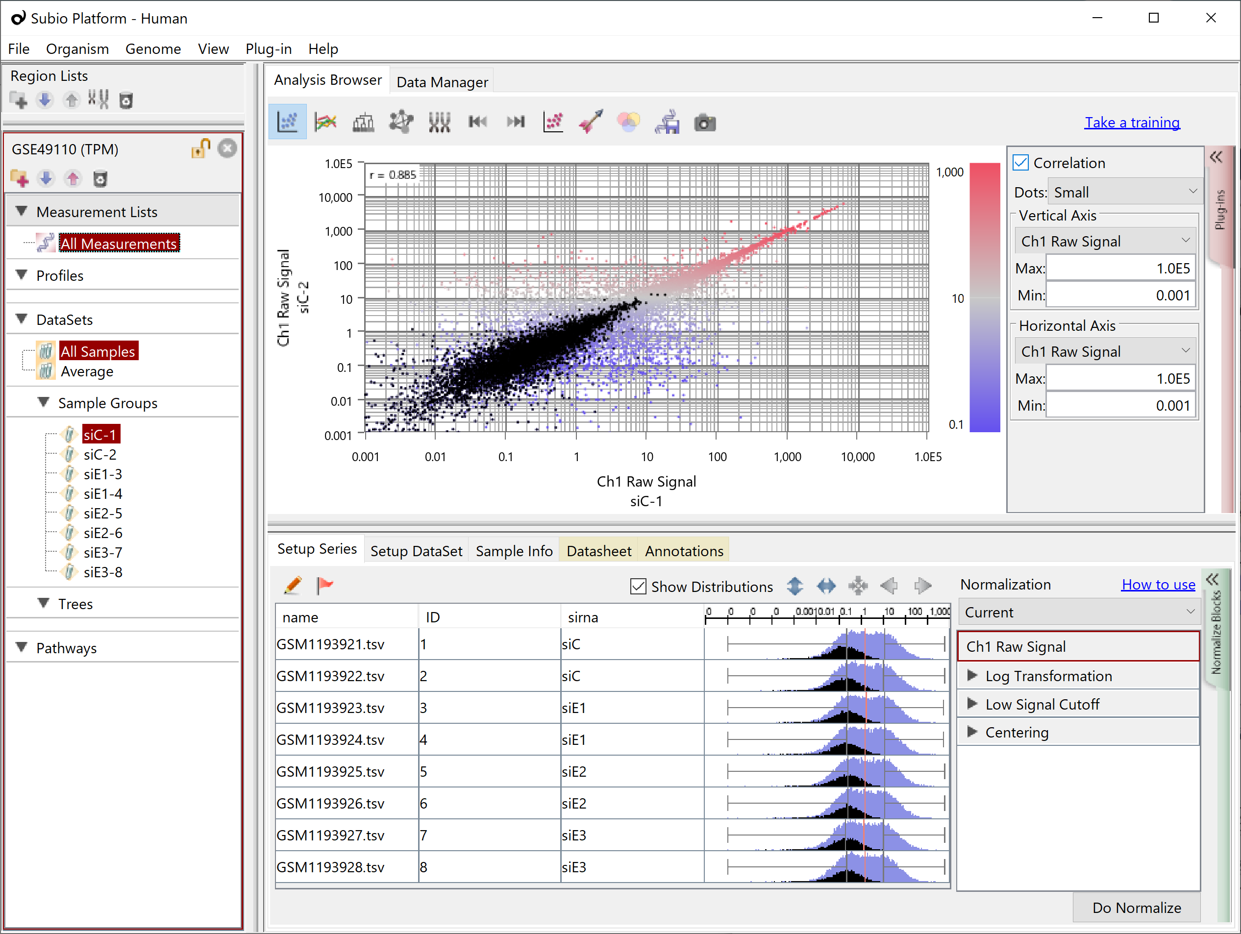
This illustrates the normalization and pre-processing of RNA-Seq data using Subio Platform . Even if you use R/Bioconductor, it is helpful to understand the concepts.
Finding a proper sequence of normalization and pre-processing.
Subio Platform offers the following normalization scenarios. You can pick one as a template and adjust the options to make it fit the characteristics of the data.
- Expression Microarray
- RNA-Seq (Count)
- RNA-Seq (FPKM, TPM, RPKM)
- Methylation Beta Values
- Pre-normalized Log2 Data - Select this if you have pre-normalized log2 ratio data.
- Nothing - Select this to clear all blocks.
Novice users might feel unconfident about the settings, but we will support them through online training so that they can learn the whole analysis process for the data they want to analyze.
When you measure the transcriptome with RNA-Seq, there are a lot of 0 (or missing values) in the table of read-counts (Counts). The difficulty with RNA-Seq data analysis is that 0 indicating no mapped read does not necessarily mean the gene is NOT-expressed.
The reason is obvious when you look at a table of Counts from replicated samples. You can easily find genes with a Count value at a sample while 0 at another. It suggests that it may not be captured by the sequencer even if expressed. It is probabilistic whether an expressed gene has a Count value or 0 by chance. The lower the expression, the higher the probability of being counted 0. We can find such genes more in the noise range.
Let's say you are comparing the average expression levels between groups A and B. You find a gene looks down-regulated in group B. However, you find some samples in group B are with 0 counts. The rest of Count values are almost the same as group A. You can easily detect false positives if you improperly treat Count 0. So, let's think about how to handle the RNA-Seq data.Let's say you are comparing the average expression levels between groups A and B. You find a gene looks down-regulated in group B. However, you find some samples in group B are with 0 counts. The rest of Count values are almost the same as group A. You can easily detect false positives if you improperly treat Count 0. So, let's think about how to handle the RNA-Seq data.
For The Count Data
If you have replicate samples and look at a scatter plot of Counts among them, you will see dots converging on the diagonal in the range of high values, but not in the low Counts'. They are the signal and noise range of the data. There is no definite boundary between them. Although the border strictly depends on the actual data set, the higher than 100 for Count often looks like the signal range, and the lower than ten often looks like the noise. And the boundary often looks lying somewhere between 10 and 100. As mentioned above, genes in the noise range have more chance of having 0 Counts. (black dots)

Therefore, Subio Platform offers a preset normalization scenario called RNA-Seq (Count) and performs the following pre-preprocessing and normalization on the Count.
- Log Transformation: base 2
- global normalization: at 90th percentile
- Low Signal Cutoff: Replace <20 to 20
- fill missing values: 4
- Centering
By Step 1, the 0 Counts turn to the missing value.
Step 2 is the global normalization, of which purpose and effect are equivalent to the normalization widely used for RNA-Seq data, dividing total mapped reads by 1 million. Dividing by 1 million can be imperfect, actually, so it is beneficial even for such normalized data to apply this redundantly. Please adjust the percentile to the data; the default is 90. The broader dynamic range allows lower value, and the narrower dynamic range restricts the percentile to high.
Step 3 is a measure to align the lower limit of Count with the lower end of the signal range to prevent falsely detecting differentially expressed genes (DEGs) due to the measurement values in the noise range.
Step 4 is to replace the missing value of Count 0 with some value. You can set the same value as in step 3, or a little lower. However, you put it with an exponent. Four, the default, means 16 (2^4), which is about half of the cutoff set in step 3.
Step 5 is what makes it a ratio to the mean of the whole sample. You can replace it with the Ratio to Control Samples block if you have the control.
If you want to examine in detail, please look at this Excel worksheet.
For The TPM/FPKM/RPKM Data
Analyzing TPM, FPKM, and RPKM data is more troublesome than in the case of Count because the noise region is spread over the signal region (black dots), and replacing 0 with some value can bring the problem of falsely detecting DEGs as mentioned at the beginning.

Let's take a look at the Subio Platform's preset normalized scenarios RNA-Seq (TPM, FPKM, RPKM).
- Log Transformation: base 2
- global normalization: at 90th percentile
- Low Signal Cutoff: Replace <0.01 to 0.01
- Centering
Up to step 2 is the same as the RNA-Seq (Count) scenario, so please refer to the description there.
Step 3 sets the lower limit value, but unlike the case of Count, it cannot cancel the effect of the noise range. The usage is minimal.
In the case of Count, the Fill Missing Values block was applied here, but in the case of TPM/FPKM/RPKM, it is better not to use it. For detecting DEGs, not only using the fold-change and P values but also extracting genes with the data lack in group A but with some measurement in group B or visa versa. Remember to take this extra work.
The explanation of Step 4 is the same as the above Centering. The caveat is that it is better not to replace it with the Ratio to Control Samples block because the measurement value can be null in the Control Samples.
However, if you do a multivariate analysis such as clustering in this state, the missing values will get in the way. So, you could add Fill Missing Values after Centering and replace it with some value that represents a decrease in expression, such as -1. Therefore, it is necessary to switch the presence or absence of Fill Missing Values between the expression difference analysis and the multivariate analysis, which also takes time.