Several tools are available for RNA-Seq deconvolution analysis, including xCell, CIBERSORTx, MCP-counter, EPIC, and quanTIseq.
However, when you actually begin an analysis, the first challenge is deciding which tool to use. Possible selection criteria include:
- What values are used as input
- Whether processing for noise, batch effects, and related issues is included
- Whether paired structure can be used in the statistical analysis
- What types of cells can be estimated
- How the resulting values can be used
- What types of figures can be produced
These are some of the points that need to be considered.
In this article, we use the paired RNA-Seq dataset GSE121212 from patients with atopic dermatitis and make each of these decisions step by step in consultation with ChatGPT. We began by comparing analysis tools, designed the preprocessing of the input data, and then asked AI to generate an R script that matched the selected conditions. We also worked with AI to correct errors encountered during execution, organize the statistical results, interpret the biological findings, and refine the visualization method.
By working through these tasks with AI, we were able to move from deciding the analysis strategy to visualizing the results in far less time than would previously have been possible.
Comparing RNA-Seq Deconvolution Analysis Tools
Several tools are available for RNA-Seq deconvolution analysis, but they do not all produce the same type of result. They differ in their estimation targets, output values, required input data, and execution methods, so the tool must be selected according to the purpose of the analysis.
| Tool | Main targets | Output | Execution environment | Main input | Advantages | Points to note |
|---|---|---|---|---|---|---|
| xCell | 64 cell types, including immune and stromal cells | Enrichment score | R, Web | An expression matrix with Gene Symbols × Samples. Gene length- and library size-adjusted values such as TPM are recommended for RNA-Seq, but normalized Gene Counts were used here according to the purpose of the analysis | Covers a broad range of cell types, including non-immune cells. Useful for exploring relative changes among samples | The output is not a cell fraction. Overlap between signatures of closely related cell types and the treatment of low-expression values require caution |
| CIBERSORTx | Mainly immune cells. Custom signatures can also be created | Relative or absolute estimates of cell abundance and cell-type-specific expression estimates | Web, Docker | Mixture expression matrix and signature matrix | Widely used and can estimate relative cell fractions or absolute abundance scores, depending on the selected mode. Custom signatures can be generated from scRNA-Seq data | Relative cell fractions, absolute abundance scores, or cell-type-specific expression estimates |
| MCP-counter | Eight immune-cell populations, endothelial cells, and fibroblasts | Abundance score | R | An expression matrix with Gene Symbols × Samples | Because the target cell populations are limited, it is useful for comparing major immune and stromal cell populations across samples | The output is not a cell fraction. The target cell populations are limited, and fine immune-cell subtypes cannot be distinguished |
| EPIC | Immune cells, fibroblasts, endothelial cells, and other cells | Cell fraction or mRNA fraction | R, Web | Bulk RNA-Seq expression matrix | Can estimate composition including non-immune cells | Designed mainly for the tumor microenvironment. When applying it to other tissues such as skin, differences from the reference must be considered |
| quanTIseq | 10 immune-cell types | Cell fractions and the fraction of uncharacterized cells | R, command line, Web | FASTQ files or an RNA-Seq expression matrix | Can be run from FASTQ files, and the output is relatively straightforward to interpret as cell fractions | Mainly targets blood and tumor immunity, and classification of non-immune cells is limited |
| immunedeconv | Multiple deconvolution methods through a unified interface | Depends on the selected method | R | Usually an expression matrix with Gene Symbols × Samples | Allows xCell, MCP-counter, EPIC, quanTIseq, and other methods to be run and compared in a common format | It is an interface to multiple methods rather than an independent deconvolution method. The differences in output among the methods must be understood |
In this analysis, our goal was first to explore a broad range of candidate changes among immune and stromal cells in skin tissue, and then compare the resulting scores within patients. We therefore selected xCell because it covers a broad range of cell types and can be run locally in R. However, xCell does not output cell fractions. It outputs enrichment scores for gene sets associated with specific cell types. This distinction requires caution when interpreting the statistical results and deciding how to visualize them.
Using AI to Decide What to Input into xCell
After selecting the tool, we considered which expression values should be entered into xCell.
AI first suggested TPM, which is commonly used as RNA-Seq input for xCell. However, because TPM does not retain information about the original read counts, it cannot be used to assess measurement precision in the low-count range.
We therefore decided, in consultation with AI, to prioritize examining the effects of the unstable dynamic range in the low-count region rather than gene-length correction, and created two inputs from normalized Gene Counts.
Input 1 consisted of Gene Counts after normalization and Log2 transformation. Entries with Counts of 0 were treated as missing values after the transformation. Because the minimum value in the normalized and Log2-transformed Gene Counts table was -0.6436, entries corresponding to Counts of 0 and entries that were originally missing were filled with -0.7.
Importantly, the lower bound of the low-count range after normalization differs among samples depending on their dynamic range. Therefore, Input 1 contains not only biological differences, but also measurement instability in the low-count range and non-biological variation reflecting differences in dynamic range among samples.
To address this issue, Input 2 was designed so that instability in the low-count range and non-biological variation would not be directly reflected in the xCell calculation.
The Low Signal Cutoff was set to 4.3219, corresponding to 20 on the linear scale, and values corresponding to Counts of 1 or more but less than 20 were replaced with 4.3219. In addition, values that were originally missing and Counts of 0 that became missing after Log2 transformation were filled with 4. The cutoff shown here was determined by examining scatter plots and is not intended to be applied unconditionally to every dataset. This prevented measurement instability in the low-count range and non-biological variation caused by differences in dynamic range among samples from being reflected in the analysis, while still distinguishing 0 or missing values from low-expression values with a Gene Count of at least 1
The normalized Gene Counts input files used in this analysis can be downloaded here.
Asking AI to Generate an R Script for the Selected Analysis Conditions
After deciding the analysis strategy, we provided AI with the input file format and the operations to be performed, and asked it to generate an R script.
The generated R script automated the following processes:
- Reading metadata and expression values
- Converting Entrez Gene IDs to Gene Symbols
- Resolving duplicated Gene Symbols
- Running xCell analysis for Input 1 and Input 2
- Welch's t-test without accounting for pairing
- Paired t-test within patients
- Multiple-testing correction
- Counting the direction of increase or decrease in each patient
- Comparing the results from Input 1 and Input 2
An error occurred during the first execution. When the error message was shown to AI, it proposed a correction, which allowed the analysis to continue.
The R script used in this analysis can be downloaded here.
In this way, AI is not merely a tool that generates code once and then stops. It can also be used as a partner for revising scripts while checking execution results and error messages.
Reviewing the Statistical Results with AI
After the analysis, we provided AI with the statistical result files for Input 1 and Input 2 and examined whether the main findings changed depending on preprocessing.
The number of xCell output categories with a paired p-value below 0.05 was 28 for Input 1 and 27 for Input 2, with 27 categories shared by both inputs. Major findings, including the changes observed in the Th2-cell score and ImmuneScore, were largely reproduced regardless of whether the Low Signal Cutoff was applied. In contrast, the paired p-value for B-cells was 0.0115 with Input 1 and 0.0609 with Input 2.
This comparison allowed us to distinguish signals that were affected by how values in the low-count range were handled from relatively stable signals that were maintained after changing the preprocessing method. If TPM alone had been used as the input, we might not have been able to determine whether the apparent statistical significance of the B-cell score depended on instability in the low-count range.
Refining the Visualization Method in Consultation with AI
We first displayed the xCell scores for each sample as stacked bar charts and showed the figure to AI to ask whether there were any problems with this approach. AI pointed out that stacked bar charts were inappropriate because xCell scores are not cell fractions, and summing the scores of multiple cell types does not represent the overall cellular composition of the tissue. Instead, AI suggested a heatmap in which the non-lesional and lesional skin samples from each patient were placed next to each other.
AI also suggested converting the values to Z-scores for each cell type. However, Z-score transformation would obscure the difference between cell types with relatively large scores and cell types that show only small fluctuations near 0. We therefore rejected this suggestion.
On the other hand, we adopted the suggestions regarding which major cell types to retain in the table and the order in which they should be displayed. We then displayed the actual xCell scores using a common color scale. To prevent a few extremely large values from determining the entire color range, the 95th percentile of all displayed values was set as the upper limit of the color scale. The resulting figure is shown below.
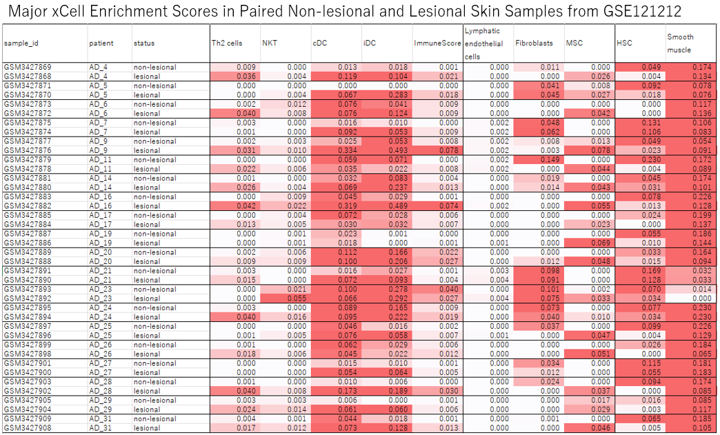
Major xCell enrichment scores calculated from Input 2 are shown for each GSE121212 sample. The non-lesional and lesional skin samples from each patient are displayed next to each other. The values shown in the cells are the actual xCell scores, and the 95th percentile of all displayed values was used as the upper limit of the color scale. However, xCell scores are not cell fractions and cannot be used to directly compare cell numbers or proportions among different cell types.
AI Makes Analysis Faster, but the Priority in Learning Shifts to Judgment
In this analysis, AI helped us compare deconvolution tools, design the input data, generate and revise an R script, review the statistical results, and improve the visualization. This allowed us to complete the workflow in far less time than would previously have been possible.
However, not every initial suggestion from AI was adopted. We chose not to use TPM alone, created two inputs to examine the effects of the low-count range, and rejected Z-score transformation for the final figure.
As AI makes coding and implementation increasingly accessible, the priority in learning data analysis should shift from spending most of the effort on writing code to understanding the entire analysis process, identifying the points that require scrutiny, and evaluating AI's initial suggestions logically and critically. This requires a broad understanding of data analysis, including the characteristics of the input values, the assumptions behind the statistical methods, the limitations of the analysis tools, and the meaning of the resulting outputs.
The main value of AI is not that it automatically determines the correct analysis, but that it allows us to examine the available options, test the analysis, and refine the results through continued dialogue.
As AI makes it possible to obtain code and results more quickly, the ability to judge whether the proposed analysis is appropriate becomes even more important.
Related Topics
edgeR & DESeq2 Analysis with ChatGPT (RNA-Seq Tutorial using R)
A New Style of RNA-Seq Data Analysis - Analyze with R/Python × Visualize and Manage Data with Subio