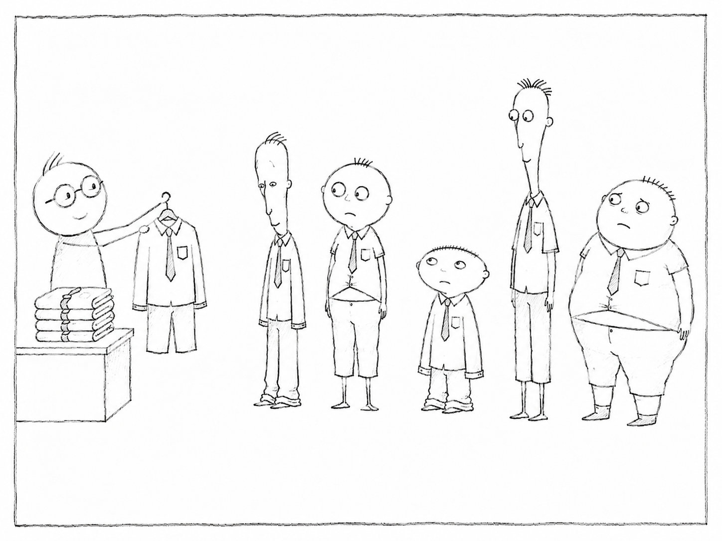
Z-score transformation can be applied to gene expression data in two fundamentally different ways.
- Gene-wise Z-scores, in which each gene is standardized across samples to show its relative expression pattern
- Sample-wise Z-score normalization, in which the values within each sample are standardized to make their distributions more comparable across samples
Gene-wise Z-scores are widely used in RNA-Seq heatmaps. The limitations of this use are discussed in detail in Why You Should Not Use Z-Scores Carelessly in RNA-Seq Heatmaps . In contrast, this article focuses on sample-wise Z-score normalization.
During the microarray era, sample-wise Z-score normalization was used to place gene expression data obtained from different samples on a common scale. However, both the values being transformed and the meaning of the transformation differ between two-color and one-color microarrays. In two-color microarrays, the signal ratio or log ratio between two samples is standardized. In one-color microarrays, the signal values of all genes measured in a single sample are standardized. Furthermore, as the number of measurable genes increased and large numbers of unexpressed and lowly expressed genes became included in the data, it became increasingly difficult to justify treating all genes as a single distribution and standardizing them using one mean and one standard deviation.
This article explains what sample-wise Z-score normalization meant in two-color microarray analysis, what changed with the transition to one-color microarrays, and what problems arise when it is applied to comprehensive gene expression datasets.
Two-color microarrays measured ratios between two samples
In early spotted two-color microarrays, two samples were labeled with Cy5 and Cy3 and measured on the same spot. The value obtained for each gene was the signal ratio between Cy5 and Cy3, or the logarithm of that ratio.
However, early spotted microarrays had many technical limitations.
- Differences in the amount of DNA deposited on each spot
- Irregularities in spot shape and position
- Local background signals
- Differences in the properties of Cy5 and Cy3 dyes
- Differences in labeling efficiency
- Differences in scanning conditions
- Signal intensity-dependent biases
Because these sources of technical variation were substantial, results obtained from different microarrays were difficult to compare without some form of normalization. Under such conditions, standardizing the center and spread of the log-ratio distribution for each microarray had practical value. Sample-wise Z-score normalization was one approach based on this rationale.
Standardizing technical variation also obscures biological variation
However, sample-wise Z-score normalization does not standardize technical variation alone. Consider, for example, a time-course experiment measuring cellular differentiation. At an early stage of differentiation, changes in the expression of most genes may be small, and the distribution of log ratios between two samples may be concentrated around zero. As differentiation progresses, many genes may become activated or repressed, causing the distribution of expression changes to become much broader.
In this case, the spread of the distribution itself is biologically meaningful, because it indicates that the transcriptional state has changed substantially during differentiation. However, if the data from each time point are transformed separately into Z-scores, both the narrow distribution at an early stage and the broad distribution at a later stage are forced to have a standard deviation of 1. As a result, small changes at early stages are relatively amplified, whereas large changes at later stages are compressed. The information that overall expression changes became larger as differentiation progressed is lost through sample-wise Z-score normalization.
Even when Z-score normalization makes data easier to compare, this does not mean that it has selectively removed measurement error alone. It standardizes technical and biological differences alike using the same transformation.
In one-color microarrays, the meaning of Z-score transformation changes
In one-color microarrays such as Affymetrix GeneChip, one sample is applied to each microarray, and a signal value is measured for each gene. Therefore, when values from a one-color microarray are transformed into Z-scores, the values being standardized are not expression ratios between two samples, but the distribution of log-transformed signal values across all genes within a single sample. This distribution is transformed to have a mean of 0 and a standard deviation of 1. Although the same term, sample-wise Z-score normalization, may be used, the biological meaning of the standardized values is fundamentally different between two-color and one-color microarrays.
Early GeneChip platforms made this approach appear somewhat reasonable
In early Affymetrix GeneChip platforms such as HG-U95, many of the technical problems that had been prominent in spotted two-color microarrays, including irregular spot formation and differences between fluorescent dyes, had been reduced.
Early GeneChip platforms measured fewer genes than later, more comprehensive microarrays. Their targets were also biased toward relatively well-characterized genes for which sequence information was available at the time. Consequently, compared with later comprehensive microarrays, the proportion of unexpressed or low-signal genes was considerably lower. In such datasets, the distribution of log-transformed signal values often appeared close to unimodal. Under these circumstances, applying sample-wise Z-score normalization to compare signal values obtained from different microarrays appeared to have some justification.
However, the fact that a distribution appears to have a single peak does not mean that different samples originally have the same gene expression distribution. Even when their histograms appear similar, differences in the centers or spreads of those distributions cannot automatically be interpreted as entirely technical.
There is no guarantee that different tissues have the same expression distribution
Consider a comparison among tissues with very different biological properties, such as brain, liver, muscle, and blood. These tissues differ both in the genes they express and in the genes they express at high levels. One tissue may express a small number of tissue-specific genes at extremely high levels, whereas another may express a larger number of genes over a broader range. There is no biological basis for assuming that the overall signal distributions of such samples are inherently the same.
Nevertheless, when each sample is transformed to have a mean of 0 and a standard deviation of 1, distributional differences arising from the biological characteristics of each tissue are also removed as though they were technical differences. Sample-wise Z-score normalization does not test whether expression distributions are the same across samples. It forcibly transforms them to have the same center and spread.
As coverage increases, the distribution no longer represents a single population
In more comprehensive microarrays, such as GeneChip HG-U133 Plus 2.0, the measured targets include not only genes that are clearly expressed in the sample, but also large numbers of probe sets corresponding to unexpressed genes or genes with signals close to the detection limit. As a result, the distribution of log-transformed signal values contains both a background or low-signal population and a population representing clearly expressed genes. Rather than forming a single peak, the distribution takes on a complex shape in which the low-signal and expressed populations overlap.
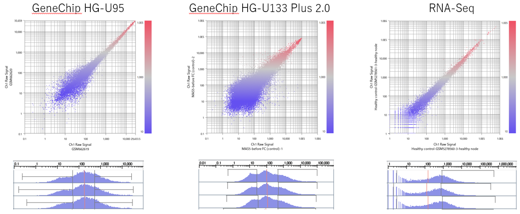
Figure: Examples of changes in gene expression value distributions
as GeneChip coverage expanded
and gene expression analysis moved toward RNA-Seq.
From left to right,
the panels show GeneChip HG-U95,
GeneChip HG-U133 Plus 2.0,
and RNA-Seq.
The upper panels show scatter plots comparing two samples,
and the lower panels show the distribution of values within each sample.
HG-U95 shows a relatively compact distribution
that is close to unimodal,
whereas HG-U133 Plus 2.0 includes more low-signal probe sets,
making the distinction between the low-signal
and expressed populations more apparent.
RNA-Seq includes even larger numbers of genes
with zero or low counts,
resulting in discrete peaks in the low-value region.
The values produced by these measurement methods
are not on the same numerical scale.
This figure is intended as a conceptual comparison
showing that, as transcriptome coverage increases,
it becomes increasingly difficult
to justify treating all genes
as a single homogeneous distribution.
Treating such a distribution as one homogeneous population and using a single mean and standard deviation to calculate Z-scores is problematic. The mean calculated from the combined populations is neither the center of the low-signal population nor the center of the expressed population. In addition, the standard deviation is strongly influenced not only by variation within each population, but also by the distance between their centers. Therefore, a Z-score calculated from this mean and standard deviation does not necessarily have a clear biological interpretation.
A Z-score can be calculated even when the original distribution is not normally distributed. However, it does not necessarily make sense to treat multiple populations with different properties as a single distribution and represent them using one mean and one standard deviation.
Quantile normalization was also introduced for one-color microarrays
For one-color microarrays, quantile normalization was introduced as a method that forces sample distributions to match more closely than sample-wise Z-score normalization does.
Sample-wise Z-score normalization sets the mean of each sample to 0 and its standard deviation to 1. In contrast, quantile normalization transforms the entire distribution of values within each sample so that all samples have the same distribution. Consequently, after quantile normalization, all samples have identical distributions when viewed as histograms. At first glance, this may appear to be a more powerful and complete form of normalization than Z-score normalization.
However, forcing distributions to match does not necessarily make gene expression data appropriately comparable.
The fundamental contradiction in quantile normalization
For quantile normalization to be valid, the observed differences in expression distributions between samples must be mainly technical, while the underlying biological expression distributions must be broadly similar.
However, this creates a fundamental contradiction. If the underlying biological distributions are already nearly the same across samples and the measurements are stable, quantile normalization will not substantially alter the data. In such datasets, there is little need to force the entire distributions to match.
In contrast, when sample distributions differ substantially and quantile normalization appears necessary, those differences may reflect not only technical factors, but also biological differences such as tissue type, cellular state, differentiation, disease, or drug response. In that situation, the assumption that the underlying expression distributions are the same no longer holds.
In other words, when the assumptions underlying quantile normalization are satisfied, strong distributional correction is unnecessary. When strong correction appears necessary, those assumptions may already have been violated.
The same problem applies to sample-wise Z-score normalization, which standardizes the mean and standard deviation. Neither method determines whether distributional differences between samples are technical or biological. They simply transform the center and spread of the distribution, or the entire distribution, without first establishing why those differences exist.
Reshaping distributions does not remove biases within the data
Even when quantile normalization makes the histograms of all samples identical, batch effects within the data are not necessarily removed. This is because batch effects do not simply increase or decrease the values of all genes uniformly. They often affect particular groups of genes, specific signal ranges, or probe sets with particular sequence characteristics. Consequently, even after the overall distributions of all samples have been made identical, PCA or clustering may still separate samples according to experimental date, reagent lot, measurement facility, or instrument, rather than biological condition.
The same applies to sample-wise Z-score normalization. Even after the mean and standard deviation have been standardized, the internal structure of the data remains, including which genes are biased and in which direction.
In the figure shown above, even if the overall sample distributions in the lower panels were transformed to have the same shape, this would not necessarily correct the gene-specific biases or internal structures visible in the upper scatter plots.
Simply standardizing sample distributions cannot remove technical biases that exist within the data.
Normalization is expected to reduce technical differences while preserving biological differences. However, a procedure that merely forces distributions to match cannot determine which differences are technical and which are biological.
As a result, technical biases that should be removed may remain, while biological differences that should be preserved may be lost. When evaluating a normalization method, the important question is not whether the distributions look neatly aligned after normalization, but whether the differences that should disappear have actually disappeared and whether the differences that should remain have been preserved.
These are no longer common normalization methods for RNA-Seq
Since RNA-Seq became widely used, sample-wise Z-score normalization and quantile normalization have not been commonly used as normalization methods for RNA-Seq. Instead, RNA-Seq generally uses methods that account for factors such as library size and RNA composition.
However, when sample-wise Z-score normalization is deliberately applied to RNA-Seq data, many of the same concerns arise as when it is applied to comprehensive microarrays such as GeneChip HG-U133 Plus 2.0.
The problem with forcing distributions to match remains unchanged
This problem can also be observed in actual RNA-Seq expression data. In the analysis example using GSE159751, quantile normalization was applied to FPKM distributions that differed substantially between samples.
After normalization, the distributions appeared to have the same shape in the histograms. However, when the data were examined by clustering, it became clear that simply forcing the distributions to match had not made the data suitable for biological comparison.
To repeat the central point, making distributions look the same and creating biologically comparable data are not the same thing.
Summary: Matching distributions is not the purpose of normalization
Sample-wise Z-score normalization had practical value in early microarray analysis, when technical variation was substantial, as a way of placing different datasets on a common scale.
However, with the transition from two-color to one-color microarrays, the meaning of the values being transformed into Z-scores changed substantially. Furthermore, as measurement platforms became more comprehensive, unexpressed and low-signal genes became mixed with clearly expressed genes, making it increasingly difficult to justify treating all genes as a single distribution.
Quantile normalization, which forces entire distributions to have the same shape, was also widely used. However, even when sample distributions were made identical, batch effects and gene-specific technical biases within the data were not necessarily removed.
The purpose of normalization is not to make sample distributions look neat and identical. It is to reduce technical differences while preserving the biological differences that are relevant to the analysis.
When sample distributions differ so greatly that a distribution-matching procedure appears necessary, the assumption that those differences can safely be removed as technical effects should itself be questioned.
Many methods have been proposed in the continuing effort to improve normalization. New methods will continue to appear and become widely used.
However, a neatly aligned histogram after normalization is not sufficient evidence that the procedure was appropriate. PCA, clustering, gene-level expression patterns, and sample information should be examined together to determine whether the differences that should have been removed have disappeared, and whether the differences that should have been preserved still remain.