Is the Noise Junk?

Paper fig04 thumb

GSE11670 is another example of HG-U133 Plus2.0 Array data with technical replicates of good quality. Dots widely scatter at lower left, indicating signals less than 100 are not reliable. Though the histograms of MAS5 look monomodal, but they're intrinsically bimodal. The peak is formed in between signals and noise, because the two components are close and gradual. Signals between 10 and 100 are less reliable, but not absolutely nonsense. You can download the SSA file to import to your Subio Platform.

Paper fig05 thumb

GSE11670 data by RMA. There is no widely scattered area at left-bottom, but it doesn't mean there is no noise and all data are signals. Intrinsic noise must exist in a biological context. If you see histograms (row3 and 4), there are high peak at left side. It only converges low signals into small range. Signals between 10 and 100 are consequently much less reliable, comparing to MAS5 data.

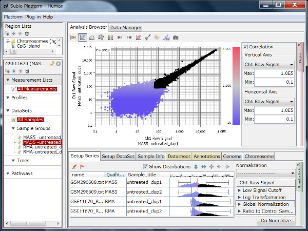
Let's say you are comparing technical replicate samples on a scatter plot. 
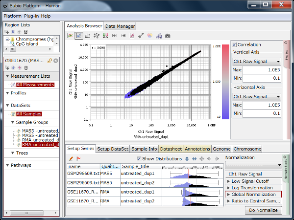
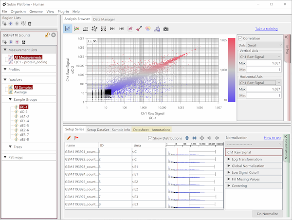
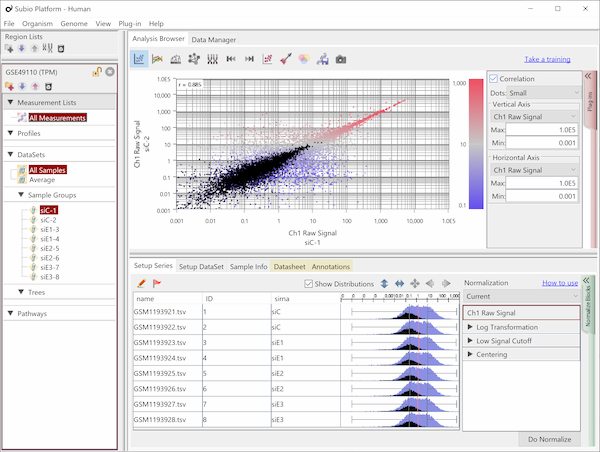
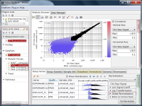
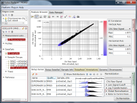
If you see charts like Fig4 and Fig5, which do you think is better quality? 
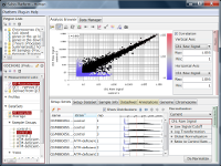
Fig4 looks varying wider partially. Correlation coefficient of Fig4 is 0.919, while that of Fig5 is 0.988. I guess many think Fig5 is better. But the two are generated from a same raw data and quantified by different algorithms, which are MAS5 (Fig4) and RMA (Fig5). For more about the characteristics of the data, please see "MAS5 vs. RMA" for more about the characteristics of the data. We focus on the reproducibility of microarray data here.

A high correlation coefficient indicates the high reproducibility. But it is not always true when you talk about microarray data. Why?

You cannot assume biologically that all genes are expressing in a sample. And every measurement system has its own dynamic range. You can rely on signals in the dynamic range (signal range), but cannot them out of the range (noise range). A microarray data must have both signals and noise. The noise is a mixture of not-expressing genes and too-low-to-detect by the system. You cannot distinguish not-expressing and too-low-to-detect from noise. So it is natural and reasonable there is an area where spots scatter widely at low signal range.

There is such a noise range in Fig4, but not in Fig5. Actually, there is the noise, which is just hidden, from a view point of experimental biology.

Hiding noise is not welcome for analysts because it makes their works difficult. If the noise range looks obvious, it is easy to set a boundary between noise and signal ranges, and extract genes with reliable signals (Fig4). But it is not easy to do it in Fig5. 
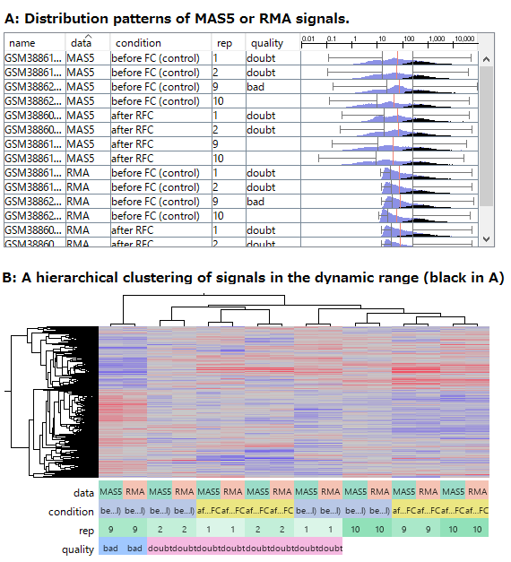
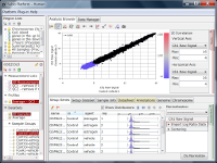
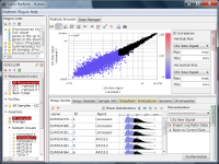
If you look closely at the histograms, there are peaks at their left ends. And if you select genes in the signal range in Fig4, the shapes of them in histograms in Fig5 look similar. So you can assume the left peaks are the noise range in Fig5, though it is hidden in the scatter plot.

A high correlation coefficient indicates the high reproducibility. This is true for signal range, but not for noise range. So a correlation coefficient calculated with all genes is not an issue. This confusion resulted in algorithms hiding noise, or treating data as if all data are in the signal range. You should clearly understand that the dynamic range is the signal range, excluding the noise range. The noise is beneficial as it looks like noise.

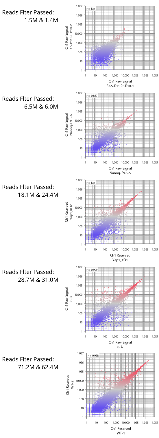
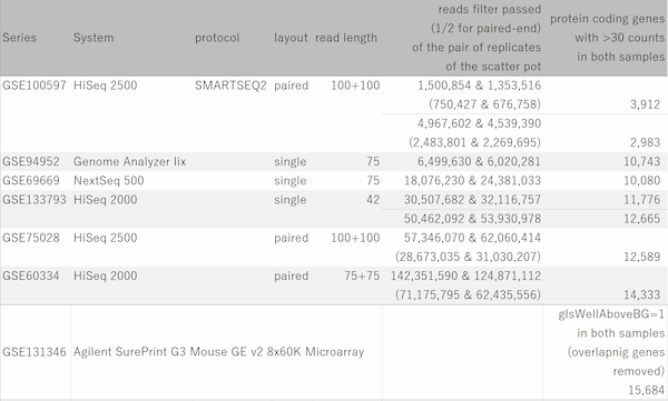
Now let's see dynamic ranges of microarray platforms.

The Dynamic Range of Microarrays

You might have heard like "4-5 orders" about the dynamic range of microarray data. But this is like saying 100km is longer than 80mi. Microarray signals depend on the hardware and software. So you cannot compare numbers from different platforms directly. You need a common unit to compare. So why don't you ask like "How many genes are reliably measured by the platform?" or "How many genes are in the signal range?"

Affymetrix 3' IVT GeneChip

This is the typical of the microarray because was massively used from 2002 to 2004. Fig4 and Fig5 are a dataset measured by Human Genome U133 Plus 2.0 Array. About 25,000 probe sets are in the signal range. Multiple probe sets are designed for some genes, so about 12,000 genes are measured reliably with this technology.

The signal and noise range are not clearly separated in actual data. The boundary is not like a line but a zone or spectrum. If the overlapping zone, or boundary zone, is large enough, it forms a peak in the histogram. You see peaks at just left of signal area (black) in Fig4. And the left skirts of peaks are noise area. Maybe you can use data in the boundary zone, if you accept the less trustfulness. You cannot separate boundary zone and noise range in RMA data (Fig5).

You can download the SSA file of GSE11670 to examine on your Subio Platform.

Illumina BeadChip

This product was released after GeneChip, and they insisted very high reproducibility. If you see a scatter plot of HumanHT-12 V4.0 expression beadchip data(Fig6), it looks ultra-low variance. But you know this is only the effect of RMA algorithm. About 15,000 probe sets are in the signal range, and about 11,000 genes are reliably measured. Notice that the dynamic range is narrower than GeneChip. The interpretation becomes difficult due to RMA, and there is no choice of quantification method.

You can download the SSA file of GSE25315 to examine on your Subio Platform.

Affymetrix Gene ST Array

Paper fig07 thumb

GSE22288 is obtained with Gene ST Array, which came after 3' IVT Array (HG-U133 Plus 2.0). 3' IVT probes are designed in 3' UTRs because those sequences are more unique than exons. Gene ST probes are targeted exon. It seems the strategy makes data more ambiguous and less sensitive. New technology is not always better than old. It's not rare that matured technology is superior in history. There are tons of 3' IVT GeneChip data available on the web,sThis is another advantage you'd better to consider. You can download the SSA file to import to your Subio Platform.

Affymetrix changed the fundamental design of 3' IVT GeneChip, and released later. MAS5 is no more available, and you can select only RMA or similar methods which hide noise. It is very difficult to distinguish signal and noise range (Fig7). In the area of >6 (log2) signal, plots are scattering wider as signals go low. This is a natural form. Unlikely, plots is converging as signals go low in the <6 signal area. This is artificial form made by the software. It is hard to divide though, about 12,000 – 15,000 probe sets, or about 9,000 – 11,000 genes are in the signal range.

If you want to know the noise range more clearly, it is a good idea to search plots of not-expressing genes in the cell or organ. You will know how broad such plots locate. Because the boundary zone is so wide that it is very difficult to interpret the data.

The newer products after GeneChip Plus2.0 have narrower dynamic range. And the latest Clariom S Array has the narrowest. The fame as a technology leader has completely faded.

You can download the SSA file of GSE22288 to examine on your Subio Platform.

Agilent Whole Genome 4x44k Microarray

Paper fig08 thumb

GSE36082 is obtained with Agilent Whole Genome 4x44k microarray, which was a great achievement of microarray technology. And their SurePrint microarrays keep the paramount quality. There is a steep peak at the left end of histogram, which is formed by signals as low as negative control probes. What's good is the edge is brilliantly sharp. It seems you might have a chance to measure slightly expressing genes, or to distinguish not- and lowly-expressing genes. You can download the SSA file to import to your Subio Platform.

The former microarrays were poor though, Agilent made a great improvement in 4x44k series in 2004. And they have kept the unparalleled dynamic range since then. In Fig8, the number of probes in the signal range reached to about 34,000, it means you can measure more than 16,000 genes with this technology. It enables your measuring expression levels of less transcribed genes, and it has more impact from a biological point of view.

The noise is a mixture of signals of not-expressing and too-low-to-detect genes. If you want to know what genes are not expressing, you must increase sensitivity to reduce the latter. So this technology gives you not only signals of 4,000 to 5,000 more genes, but also purer list of not-expressing genes. So this is only the technology for studies of ON/OFF behaviors of genes.

You can download the SSA file of GSE36082 to examine on your Subio Platform.

Microarray vs. RNA-Seq

The dynamic range of RNA-Seq theoretically depends on the number of reads. And practically, 20-50 million reads are comparable to the Affymetrix 3' IVT GeneChip. And to rival Agilent's microarrays, we would expect you need about 100 million reads (200 million if paired-end).

What Is the "Good" Expression Data?

As mentioned above, the dynamic range and data characteristics vary among microarray systems. If you want to analyze the highly expressed 10,000 to 12,000 genes, you can generally choose any platform. However, if you need to investigate the 4,000-5,000 genes with lower expression levels than that as well, there is no other option but Agilent's microarrays.

There is no measurement data without noise. If it looks to have no noise, we need to consider why this is the case and investigate the invisible boundary between the signal and noise ranges. This is very difficult to do. Therefore, good data refers to data that is easy to analyze and produces highly reliable analysis results, which means that it has the following characteristics.

  • The noise is visible as noise.
  • There are many genes in the signal range.
  • There is little overlap between the signal and noise ranges.
  • It is highly sensitive to detect differences in the expression levels.

We haven't mentioned the fourth point before. Data processing methods like RMA reduce not only the variability between samples but also the sensitivity for detecting differences of the expression levels. If you expect small differences in the study subjects, keep this in mind and choose the right platform.

The Solution We Offer, Subio Platform

Banner epilogue

Nobody knows how to handle omics data. Nobody knows how to extract meaning from omics data. We think it is not statisticians or bioinformaticians, but is an experimental biologist who will bring a critical idea someday. So it is essential to invite them to the table of discussion, at where everybody is equally amateur.

Please read why we create Subio Platform software, and what we offer to you who challenge the indeterminate problem.

Please read the following articles, too.

Back to Top